Spatial Data - Displaying time series, spatial and space-time data with R
Table of Contents
1. Proportional symbol mapping

1.1. Interactive Graphics
1.1.1. mapView


1.1.2. rgl

2. Choropleth maps


3. Cartogram

4. Raster maps

4.1. Interactive Graphics
5. Vector fields
6. Physical maps
7. Reference maps
8. Code
8.1. Proportional symbol mapping
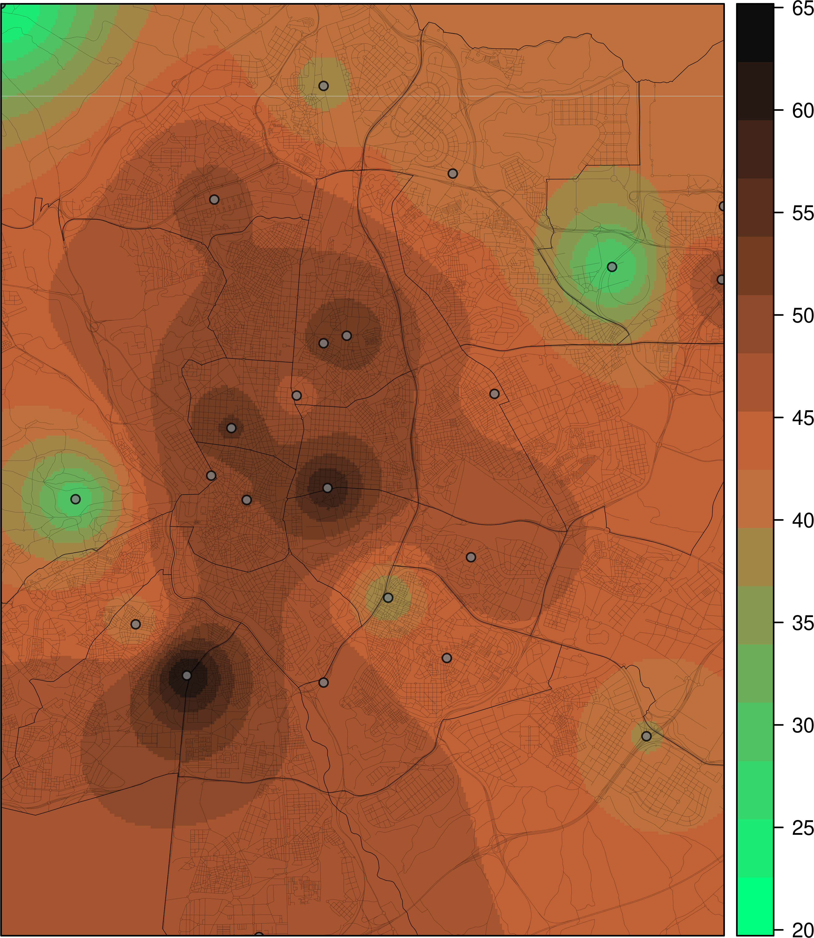
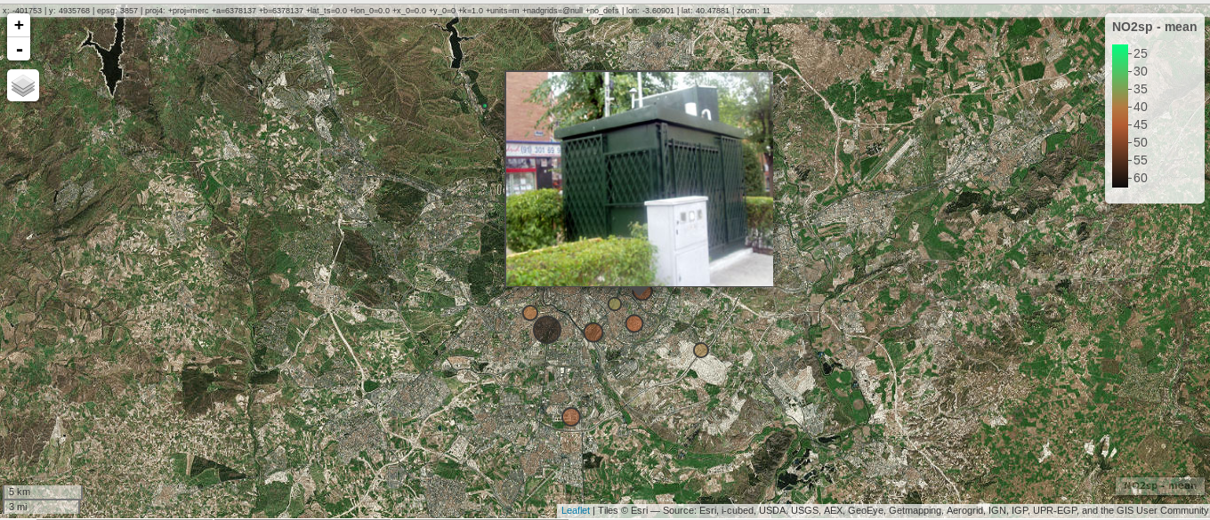
##################################################################
## Initial configuration
##################################################################
## Clone or download the repository and set the working directory
## with setwd to the folder where the repository is located.

library("lattice")
library("ggplot2")
## latticeExtra must be loaded after ggplot2 to prevent masking of its
## `layer` function.
library("latticeExtra")

library("RColorBrewer")

source("configLattice.R")
##################################################################

library("sp")
library("sf")

NO2sf <- st_read(dsn = "data/Spatial/", layer = "NO2sf")

airPal <- colorRampPalette(c("springgreen1", "sienna3", "gray5"))(5)

##################################################################
## Proportional symbol: ggplot
##################################################################

## Create a categorical variable
NO2sf$Mean <- cut(NO2sf$mean, 5)

ggplot(data = NO2sf) +
    geom_sf(aes(size = Mean, fill = Mean),
            pch = 21, col = 'black') +
    scale_fill_manual(values = airPal) +
    theme_bw()

##################################################################
## Proportional symbol: sppplot
##################################################################

NO2sp <- as(NO2sf, "Spatial")

spplot(NO2sp["mean"],
       col.regions = airPal, ## Palette
       cex = sqrt(1:5), ## Size of circles
       edge.col = "black", ## Color of border
       scales = list(draw = TRUE), ## Draw scales
       key.space = "right") ## Put legend on the right

##################################################################
## Optimal classification and sizes to improve discrimination
##################################################################

library("classInt")
## The number of classes is chosen between the Sturges and the
## Scott rules.
nClasses <- 5
intervals <- classIntervals(NO2sp$mean, n = nClasses, style = "fisher")
## Number of classes is not always the same as the proposed number
nClasses <- length(intervals$brks) - 1

op <- options(digits = 4)
tab <- print(intervals)
options(op)

## Complete Dent set of circle radii (mm)
dent <- c(0.64, 1.14, 1.65, 2.79, 4.32, 6.22, 9.65, 12.95, 15.11)
## Subset for our dataset
dentAQ <- dent[seq_len(nClasses)]
## Link Size and Class: findCols returns the class number of each
## point; cex is the vector of sizes for each data point
idx <- findCols(intervals)
cexNO2 <- dentAQ[idx]

## spplot version
NO2sp$classNO2 <- factor(names(tab)[idx])

## Definition of an improved key with title and background
NO2key <- list(x = 0.99, y = 0.01, corner = c(1, 0),
               title = expression(NO[2]~~(paste(mu, plain(g))/m^3)),
               cex.title = 0.8, cex = 1,
               background = "gray92")

pNO2 <- spplot(NO2sp["classNO2"],
               col.regions = airPal,
               cex = dentAQ * 0.8,
               edge.col = "black",
               scales = list(draw = TRUE),
               key.space = NO2key)
pNO2

## ggplot2 version
NO2sf$classNO2 <- factor(names(tab)[idx])

ggplot(data = NO2sf) +
    geom_sf(aes(size = classNO2, fill = classNO2),
            pch = 21, col = "black") +
    scale_fill_manual(values = airPal) +
    scale_size_manual(values = dentAQ * 2)  +
    xlab("") + ylab("") + theme_bw()

##################################################################
## Spatial context with underlying layers and labels
##################################################################

##################################################################
## OpenStreetMap
##################################################################

library("osmdata")

madridBox <- st_bbox(NO2sf)

qosm <- opq(madridBox) %>%
  add_osm_feature(key = "highway",
                  value = "residential")

qsf <- osmdata_sf(qosm)

library("ggrepel")

ggplot()+
  ## Layers are drawn sequentially, so the NO2sf layer must be in
  ## the last place to be on top
  geom_sf(data = qsf$osm_lines["name"],
          size = 0.3,
          color = "lightgray") +
  geom_sf(data = NO2sf,
          aes(size = classNO2,
              fill = classNO2),
          pch = 21, col = "black") +
  ## Labels for each point, with position according to the circle size
  ## and the rest of labels
  geom_text_repel(data = NO2sf,
                  aes(label = substring(codEst, 7),
                      geometry = geometry,
                      point.size = classNO2),
                  stat = "sf_coordinates") +
  scale_fill_manual(values = airPal) +
  scale_size_manual(values = dentAQ * 2) +
  labs(x = NULL, y = NULL) + theme_bw()

qsp <- osmdata_sp(qosm)

qspLines <- list("sp.lines", qsp$osm_lines["name"],
                 lwd = 0.1)

spplot(NO2sp["classNO2"],
       col.regions = airPal,
       cex = dentAQ,
       edge.col = "black",
       alpha = 0.8,
       sp.layout = qspLines,
       scales = list(draw = TRUE),
       key.space = NO2key)

##################################################################
## Shapefiles
##################################################################

## Madrid districts
unzip("data/Spatial/distr2022.zip", exdir = tempdir())

distritosMadridSF <- st_read(dsn = tempdir(),
                             layer = "dist2022")
## Filter the streets of the Municipality of Madrid
distritosMadridSF <- distritosMadridSF[distritosMadridSF$CMUN == "079",]
## Assign the geographical reference
distritosMadridSF <- st_transform(distritosMadridSF,
                                  crs = "WGS84")

## Madrid streets
unzip("data/Spatial/call2022.zip", exdir = tempdir())

streetsMadridSF <- st_read(dsn = tempdir(),
                           layer = "Gdie_g_calles")
streetsMadridSF <- streetsMadridSF[streetsMadridSF$CDMUNI == "079",]
streetsMadridSF <- st_transform(streetsMadridSF,
                                crs = "WGS84")

ggplot()+
  geom_sf(data = streetsMadridSF,
          size = 0.1,
          color = "darkgray") +
  geom_sf(data = distritosMadridSF,
          fill = "lightgray",
          alpha = 0.2,
          size = 0.15,
          color = "black") +
  geom_sf(data = NO2sf,
          aes(size = classNO2,
              fill = classNO2),
          pch = 21, col = "black") +
  geom_text_repel(data = NO2sf,
                  aes(label = substring(codEst, 7),
                      geometry = geometry,
                      point.size = classNO2),
                  size = 2.5,
                  stat = "sf_coordinates") +
  scale_fill_manual(values = airPal) +
  scale_size_manual(values = dentAQ * 2) +
  labs(x = NULL, y = NULL) + theme_bw()

distritosMadridSP <- as(distritosMadridSF, "Spatial")
streetsMadridSP <- as(streetsMadridSF, "Spatial")
## Lists using the structure accepted by sp.layout, with the polygons,
## lines, and points, and their graphical parameters
spDistricts <- list("sp.polygons", distritosMadridSP,
                    fill = "gray97", lwd = 0.3)
spStreets <- list("sp.lines", streetsMadridSP,
                  lwd = 0.05)

## spplot with sp.layout version
spplot(NO2sp["classNO2"],
       col.regions = airPal,
       cex = dentAQ,
       edge.col = "black",
       alpha = 0.8,
       sp.layout = list(spDistricts, spStreets),
       scales = list(draw = TRUE),
       key.space = NO2key)

## lattice with layer version
pNO2 +
    ## Polygons and lines *below* (layer_) the figure
    layer_(
    {
        sp.polygons(distritosMadridSP,
                    fill = "gray97",
                    lwd = 0.3)
        sp.lines(streetsMadridSP,
                 lwd = 0.05)
    })

##################################################################
## Spatial interpolation
##################################################################

library("gstat")

## Sample 10^5 points locations within the bounding box of NO2sp using
## regular sampling
airGrid <- spsample(NO2sp, type = "regular", n = 1e5)
## Convert the SpatialPoints object into a SpatialGrid object
gridded(airGrid) <- TRUE
## Compute the IDW interpolation
airKrige <- krige(mean ~ 1, NO2sp, airGrid)

spplot(airKrige["var1.pred"], ## Variable interpolated
       col.regions = colorRampPalette(airPal)) +
  layer({ ## Overlay boundaries and points
    sp.polygons(distritosMadridSP,
                fill = "transparent",
                lwd = 0.3)
    sp.lines(streetsMadridSP,
             lwd = 0.07)
    sp.points(NO2sp,
              pch = 21,
              alpha = 0.8,
              fill = "gray50",
              col = "black")
  })

##################################################################
## Interactive graphics
##################################################################

##################################################################
## mapView
##################################################################

library("mapview")

pal <- colorRampPalette(c("springgreen1", "sienna3", "gray5"))

mapview(NO2sp,
        zcol = "mean", ## Variable to display
        cex = "mean", ## Use this variable for the circle sizes
        col.regions = pal,
        label = NO2sp$Name,
        legend = TRUE)

##################################################################
## Tooltips with images and graphs
##################################################################

library("leafpop")

img <- paste("images/Spatial/", NO2sp$codEst, ".jpg", sep = "")

mapview(NO2sp,
        zcol = "mean",
        cex = "mean",
        col.regions = pal,
        label = NO2sp$Name,
        popup = popupImage(img, src = "local", embed = TRUE),
        map.type = "Esri.WorldImagery",
        legend = TRUE)

## Read the time series
airQuality <- read.csv2("data/Spatial/airQuality.csv")
## We need only NO2 data (codParam 8)
NO2 <- subset(airQuality, codParam == 8)
## Time index in a new column
NO2$tt <- with(NO2,
               as.Date(paste(year, month, day, sep = "-")))
## Stations code
stations <- unique(NO2$codEst)
## Loop to create a scatterplot for each station.
pList <- lapply(stations,
                function(i)
                    xyplot(dat ~ tt, data = NO2,
                           subset = (codEst == i),
                           type = "l",
                           xlab = "", ylab = "")
                )

mapview(NO2sp,
        zcol = "mean",
        cex = "mean",
        col.regions = pal,
        label = NO2sp$Name,
        popup = popupGraph(pList),
        map.type = "Esri.WorldImagery",
        legend = TRUE)

##################################################################
## Synchronise multiple graphics
##################################################################

library("leafsync")

## Map of the average value
mapMean <- mapview(NO2sp, zcol = "mean", cex = "mean",
                   col.regions = pal, legend = TRUE,
                   map.types = "OpenStreetMap.Mapnik",
                   label = NO2sp$Name)

## Map of the median
mapMedian <- mapview(NO2sp, zcol = "median", cex = "median",
                     col.regions = pal, legend = TRUE,
                     #map.type = "NASAGIBS.ViirsEarthAtNight",
                     label = NO2sp$Name)

## Map of the standard deviation
mapSD <- mapview(NO2sp, zcol = "sd", cex = "sd",
                 col.regions = pal, legend = TRUE,
                 map.type = "Esri.WorldImagery",
                 label = NO2sp$Name)

## All together
sync(mapMean, mapMedian, mapSD, ncol = 3)

##################################################################
## GeoJSON and OpenStreepMap
##################################################################

st_write(NO2sf,
         dsn = "data/Spatial/NO2.geojson",
         layer = "NO2sp",
         driver = "GeoJSON")

##################################################################
## Keyhole Markup Language
##################################################################

st_write(NO2sf,
         dsn = "data/Spatial/NO2_mean.kml",
         layer = "mean",
         driver = "KML")

##################################################################
## 3D visualization
##################################################################

library("rgl")

## rgl does not understand Spatial* objects
NO2df <- as.data.frame(NO2sp)

## Color of each point according to its class
airPal <- colorRampPalette(c("springgreen1", "sienna3", "gray5"))(5)
colorClasses <- airPal[NO2df$classNO2]

plot3d(x = NO2df$coords.x1,
       y = NO2df$coords.x2,
       z = NO2df$alt,
       xlab = "Longitude",
       ylab = "Latitude",
       zlab = "Altitude",
       type = "s",
       col = colorClasses,
       radius = NO2df$mean/10)
8.2. Choropleth maps
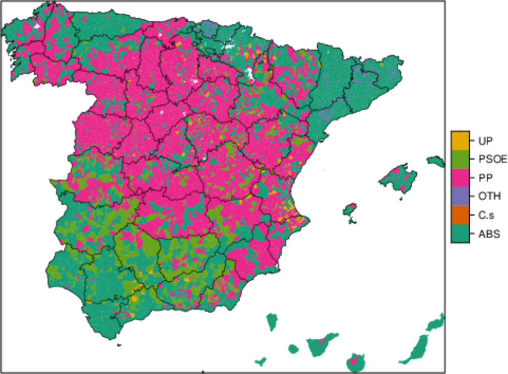
##################################################################
## Initial configuration
##################################################################
## Clone or download the repository and set the working directory
## with setwd to the folder where the repository is located.

library("lattice")
library("ggplot2")
## latticeExtra must be loaded after ggplot2 to prevent masking of its
## `layer` function.
library("latticeExtra")

library("RColorBrewer")

source("configLattice.R")
##################################################################

library("sp")

library("sf")

##################################################################
## Read data
##################################################################

sfMapVotes <- st_read("data/Spatial/sfMapVotes.shp")

sfMapVotes$whichMax <- factor(sfMapVotes$whichMax)
sfMapVotes$PROV <- factor(sfMapVotes$PROV)

summary(sfMapVotes)

##################################################################
## Province Boundaries
##################################################################

sfProvs <- st_read("data/Spatial/spain_provinces.shp",
                   crs = 25830)

##################################################################
## Quantitative variable
##################################################################

## Number of intervals (colors)
N <- 6
## Sequential palette
quantPal <- brewer.pal(n = N, "Oranges")

ggplot(sfMapVotes) +
  ## Display the pcMax variable...
  geom_sf(aes(fill = pcMax),
          ## without drawing municipality boundaries
          color = "transparent") +
  scale_fill_gradientn(colours = quantPal) +
  ## And overlay provinces boundaries
  geom_sf(data = sfProvs,
          fill = 'transparent',
          ## but do not include them in the legend
          show.legend = FALSE) +
  theme_bw()

spMapVotes <- as(sfMapVotes, "Spatial")
spProvs <- as(sfProvs, "Spatial")

## Number of cuts
ucN <- 1000
## Palette created with interpolation
ucQuantPal <- colorRampPalette(quantPal)(ucN)

## Province boundaries
provinceLines <- list("sp.polygons",
                      spProvs,
                      lwd = 0.1,
                      # draw the lines after the data
                      first = FALSE)

## Main plot
spplot(spMapVotes["pcMax"],
       col.regions = ucQuantPal,
       cuts = ucN,
       ## Do not draw municipality boundaries
       col = "transparent",
       ## Overlay province boundaries
       sp.layout = provinceLines)

##################################################################
## Data classification
##################################################################

ggplot(as.data.frame(spMapVotes),
       aes(pcMax,
           fill = whichMax,
           colour = whichMax)) +
    geom_density(alpha = 0.1) +
    theme_bw()

library("classInt")

## Compute intervals with the same number of elements
intQuant <- classIntervals(sfMapVotes$pcMax,
                           n = N, style = "quantile")
## Compute intervals with the natural breaks algorithm
intFisher <- classIntervals(sfMapVotes$pcMax,
                            n = N, style = "fisher")

plot(intQuant, pal = quantPal, main = "")

plot(intFisher, pal = quantPal, main = "")

## spplot solution

## Add a new categorical variable with cut, using the computed breaks
spMapVotes$pcMaxInt <- cut(spMapVotes$pcMax,
                           breaks = intFisher$brks,
                           include.lowest = TRUE)

spplot(spMapVotes["pcMaxInt"],
       col = "transparent",
       col.regions = quantPal,
       sp.layout = provinceLines)

## sf and geom_sf
sfMapVotes$pcMaxInt <- cut(sfMapVotes$pcMax,
                           breaks = intFisher$brks,
                           include.lowest = TRUE)

ggplot(sfMapVotes) +
  geom_sf(aes(fill = pcMaxInt),
          color = "transparent") +
  scale_fill_brewer(palette = "Oranges") +
  geom_sf(data = sfProvs,
          fill = "transparent",
          show.legend = FALSE) +
  theme_bw()

##################################################################
## Qualitative variable
##################################################################

classes <- levels(spMapVotes$whichMax)
nClasses <- length(classes)

qualPal <- brewer.pal(nClasses, "Dark2")

## spplot solution
spplot(spMapVotes["whichMax"],
       col.regions = qualPal,
       col = 'transparent',
       sp.layout = provinceLines)

## geom_sf solution
ggplot(sfMapVotes) +
  geom_sf(aes(fill = whichMax),
          color = "transparent") +
  scale_fill_brewer(palette = "Dark2") +
  geom_sf(data = sfProvs,
          fill = "transparent",
          show.legend = FALSE) +
  theme_bw()

##################################################################
## Small multiples
##################################################################

ggplot(sfMapVotes) +
  geom_sf(aes(fill = pcMaxInt),
          color = "transparent") +
  ## Define the faceting using two rows
  facet_wrap(~whichMax, nrow = 2) +
  scale_fill_brewer(palette = "Oranges") +
  geom_sf(data = sfProvs,
          fill = "transparent",
          size = 0.1,
          show.legend = FALSE) +
  theme_bw()

##################################################################
## Bivariate map
##################################################################

## PP and Cs -> Right
## PSOE and UP -> Left
levels(sfMapVotes$whichMax) <-
  c("ABS", "Right", "OTH", "Right", "Left", "Left")

## Number of steps.
Nint <- 4
## ABS - Greys, Right - Blues, OTH - Greens, Left - Reds
multiPal <- lapply(c("Greys", "Blues", "Greens", "Reds"),
                   function(pal) brewer.pal(Nint, pal))
multiPal <- do.call(rbind, multiPal)

library("biscale")


sfClass <- bi_class(sfMapVotes,
               x = whichMax,
               y = pcMax,
               style = "fisher",
               dim = 4)

bipal <- c(multiPal)

nms <- outer(1:4, 1:4, paste, sep = "-")
names(bipal) <- c(nms)

bilegend <- bi_legend(pal = bipal,
                      dim = 4,
                      xlab = "ABS-Right-OTH-Left",
                      ylab = "% of votes ",
                      size = 8)

bimap <- ggplot() +
  geom_sf(data = sfClass,
          aes(fill = bi_class),
          color = "white",
          size = 0.1,
          show.legend = FALSE) +
  bi_scale_fill(pal = bipal, dim = 4) +
  bi_theme()

library("cowplot")

ggdraw() +
  draw_plot(bimap, 0, 0, 1, 1) +
  draw_plot(bilegend, 0.05, 0.1,
            width = 0.2, height = 0.2)

## Define the intervals
intFisher <- classIntervals(spMapVotes$pcMax,
                            n = Nint, style = "fisher")
## ... and create a categorical variable with them
spMapVotes$pcMaxInt <- cut(spMapVotes$pcMax,
                           breaks = intFisher$brks)

levels(spMapVotes$whichMax) <-
  c("ABS", "Right", "OTH", "Right", "Left", "Left")

classes <- levels(spMapVotes$whichMax)
nClasses <- length(classes)

pList <- lapply(1:nClasses, function(i)
{
  ## Only those polygons corresponding to a level are selected
  mapClass <- subset(spMapVotes,
                     whichMax == classes[i])
  ## Palette
  pal <- multiPal[i, ]
  ## Produce the graphic
  pClass <- spplot(mapClass, "pcMaxInt",
                   col.regions = pal,
                   col = "transparent",
                   colorkey = FALSE)
})
names(pList) <- classes
p <- Reduce("+", pList)

op <- options(digits = 4)
tabFisher <- print(intFisher)
intervals <- names(tabFisher)
options(op)

library("grid")

legend <- layer(
{
    ## Position of the legend
    x0 <- 1000000
    y0 <- 4200000
    ## Width of the legend
    w <- 120000
    ## Height of the legend
    h <- 100000
    ## Colors
    grid.raster(multiPal, interpolate = FALSE,
                x = unit(x0, "native"),
                y = unit(y0, "native"),
                width = unit(w, "native"),
                height = unit(h, "native"))
    ## x-axis (quantitative variable)
    Ni <- length(intervals)
    grid.text(intervals,
              y = unit(y0 - 1.25 * h/2, "native"),
              x = unit(seq(x0 - w * (Ni -1)/(2*Ni),
                           x0 + w * (Ni -1)/(2*Ni),
                           length = Ni),
                       "native"),
              just = "top",
              rot = 45,
              gp = gpar(fontsize = 6))
    ## y-axis (qualitative variable)
    grid.text(classes,
              y = unit(seq(y0 + h * (nClasses -1)/(2*nClasses),
                           y0 - h * (nClasses -1)/(2*nClasses),
                           length = nClasses),
                       "native"),
              x = unit(x0 + w/2, "native"),
              just = "left",
              gp = gpar(fontsize = 6))
})

## Main plot
p + legend

##################################################################
## Interactive Graphics
##################################################################

library("mapview")

sfMapVotes0 <- st_read("data/Spatial/sfMapVotes0.shp",
                       crs = 25830)

## Quantitative variable, pcMax
mapView(sfMapVotes0,
        zcol = "pcMax", ## Choose the variable to display
        legend = TRUE,
        col.regions = quantPal)

## Qualitative variable, whichMax
mapView(sfMapVotes0,
        zcol = "whichMax",
        legend = TRUE,
        col.regions = qualPal)
8.3. Cartogram maps
##################################################################
## Initial configuration
##################################################################
## Clone or download the repository and set the working directory
## with setwd to the folder where the repository is located.

##################################################################

library("ggplot2")
library("sf")
library("cartogram")

sfPopGDPSpain <- st_read("data/Spatial/sfPopGDPSpain.shp")

ggplot(sfPopGDPSpain) +
  geom_point(aes(y = Province, x = Population/1e6)) +
  xlab("Population (million)") +
  theme_bw()

ggplot(sfPopGDPSpain) +
  geom_point(aes(y = Province, x = GDP/1e6)) +
  xlab("GDP (million euros)") +
  theme_bw()

ggplot(sfPopGDPSpain, aes(y = Population/1e6, x = GDP/1e6)) +
  geom_point() +
  geom_smooth() +
  xlab("GDP (million euros)") + ylab("Population (million)") +
  theme_bw()

cartPopNCont <- cartogram_ncont(sfPopGDPSpain, weight = "Population")

ggplot(cartPopNCont) +
  geom_sf(aes(fill = Population)) +
  scale_fill_distiller(palette = "Blues", direction = 1) +
  theme_bw()

cartGDPNCont <- cartogram_ncont(sfPopGDPSpain, weight = "GDP")

ggplot(cartGDPNCont) +
  geom_sf(aes(fill = GDP)) +
  scale_fill_distiller(palette = "Blues", direction = 1) +
  theme_bw()

cartPopCont <- cartogram_cont(sfPopGDPSpain,
                              weight = "Population")

ggplot(cartPopCont) +
  geom_sf(aes(fill = Population)) +
  scale_fill_distiller(palette = "Blues", direction = 1) +
  theme_bw()

cartGDPCont <- cartogram_cont(sfPopGDPSpain,
                              weight = "GDP")

ggplot(cartPopCont) +
  geom_sf(aes(fill = GDP)) +
  scale_fill_distiller(palette = "Blues", direction = 1) +
  theme_bw()

cartPopDorl <- cartogram_dorling(sfPopGDPSpain, weight = "Population")

ggplot(cartPopDorl) +
  geom_sf(aes(fill = Population)) +
  scale_fill_distiller(palette = "Blues", direction = 1) +
  theme_bw()

cartGDPDorl <- cartogram_dorling(sfPopGDPSpain, weight = "GDP")

ggplot(cartGDPDorl) +
  geom_sf(aes(fill = GDP)) +
  scale_fill_distiller(palette = "Blues", direction = 1) +
  theme_bw()
8.4. Raster maps
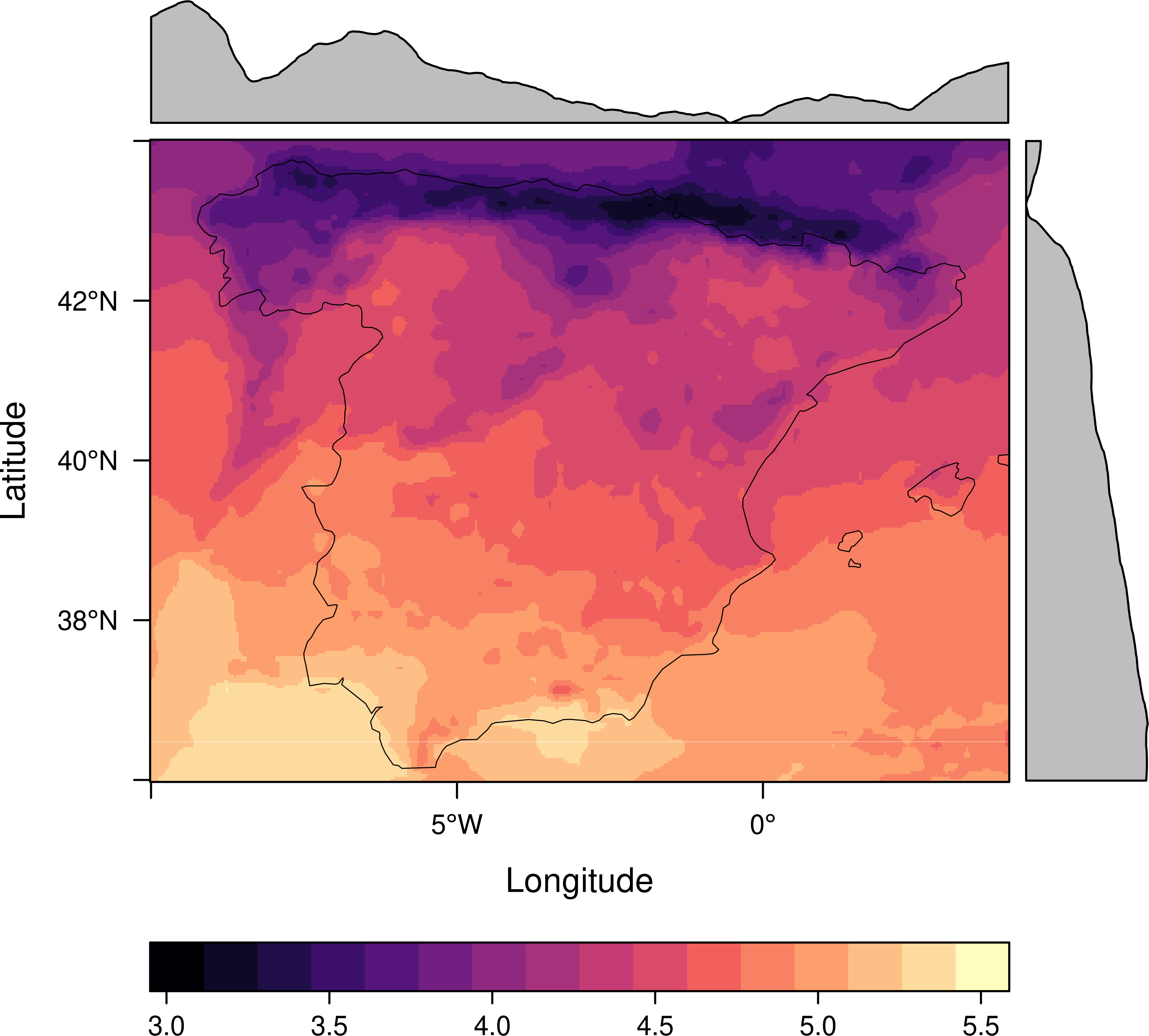
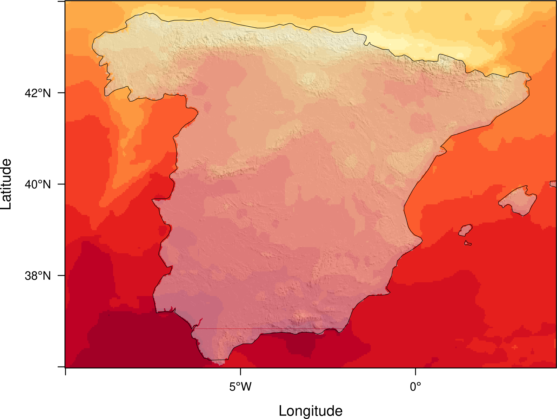
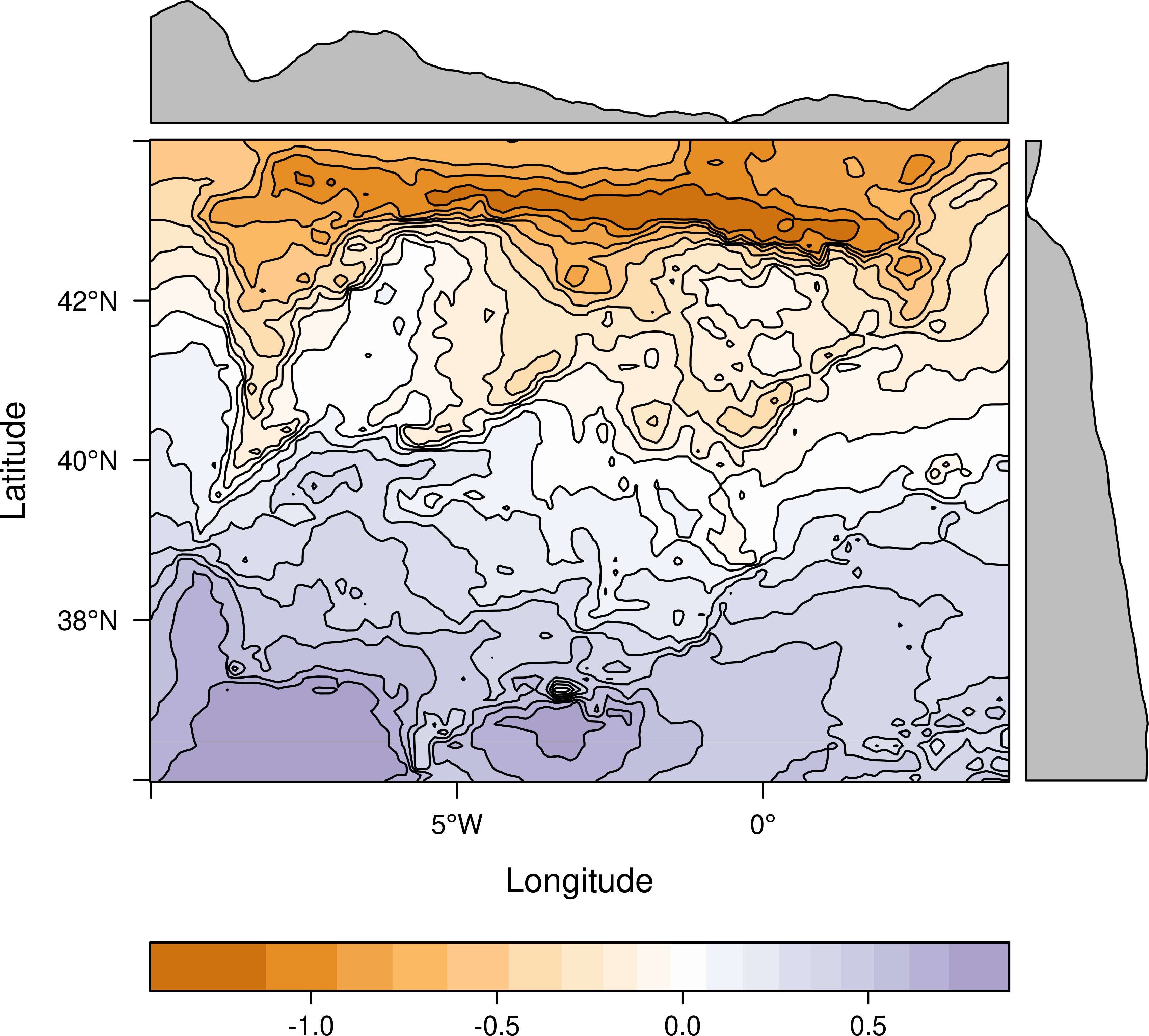
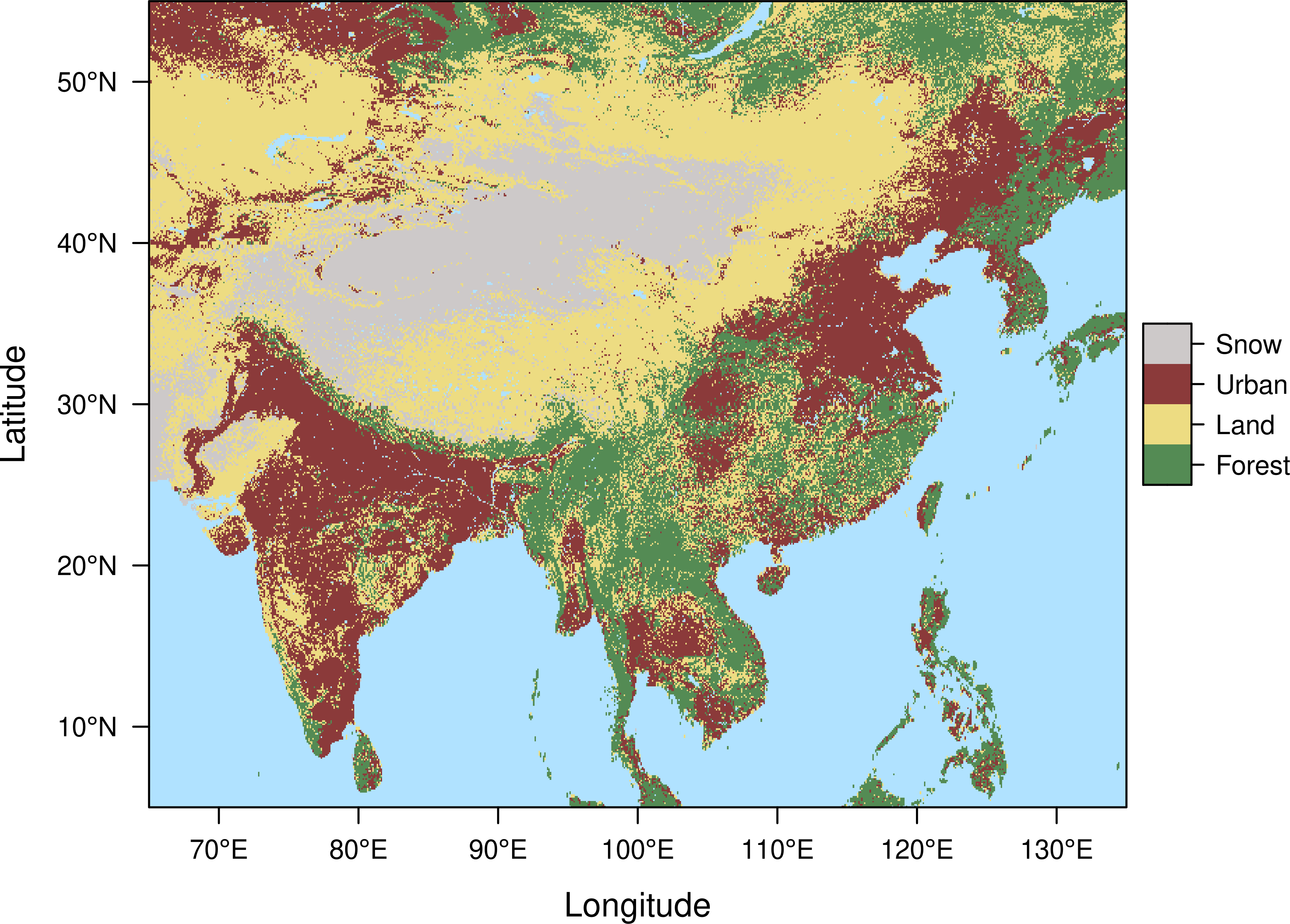
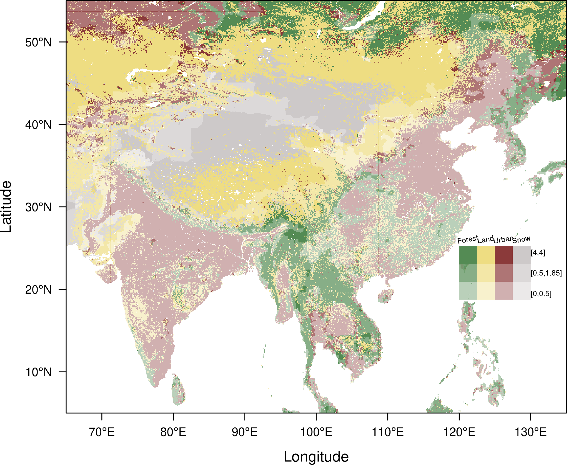
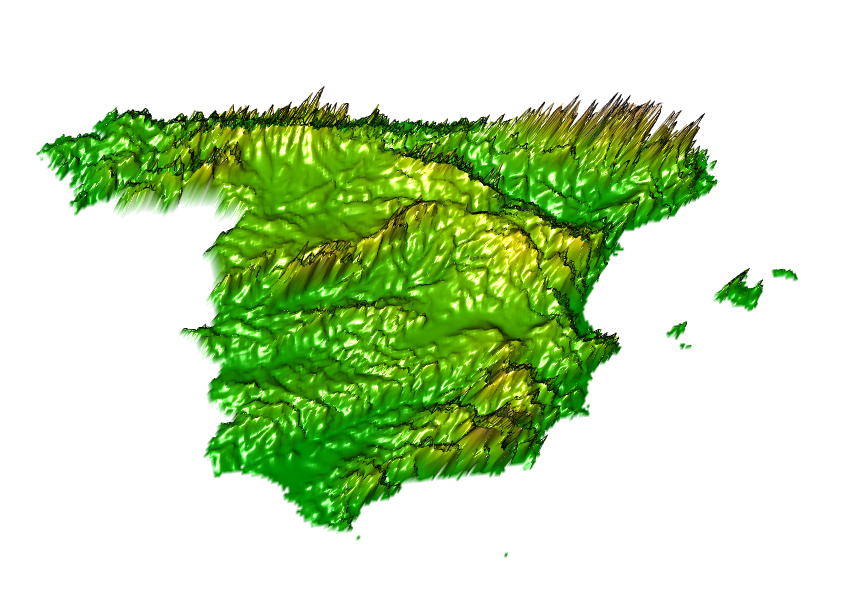
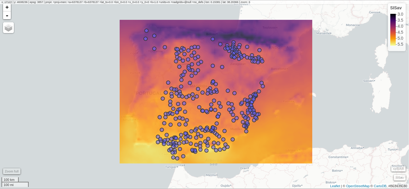
##################################################################
## Initial configuration
##################################################################
## Clone or download the repository and set the working directory
## with setwd to the folder where the repository is located.
library("lattice")
library("ggplot2")
## latticeExtra must be loaded after ggplot2 to prevent masking of its
## `layer` function.
library("latticeExtra")

library("RColorBrewer")

source("configLattice.R")

##################################################################
## Quantitative data
##################################################################

library("raster")
library("terra")
library("sf")

library("rnaturalearth")
library("geodata")

library("viridisLite")

library("rasterVis")

SISavr <- raster("data/Spatial/SISav.nc")

SISavt <- rast("data/Spatial/SISav.nc")

levelplot(SISavr)

boundarySF <- ne_countries(country = "spain", scale = 50)
## Crop to the limits of the raster object
boundarySF <- st_crop(boundarySF,
                      xmin = xmin(SISavt), ymin = ymin(SISavt),
                      xmax = xmax(SISavt), ymax = ymax(SISavt))

##ggplot2 version
gplot(SISavt) +
  geom_sf(data = boundarySF, fill = "transparent")

## lattice version
## Convert the sf object to sp
boundarySP <- as(boundarySF, "Spatial")

## Display the data ...
levelplot(SISavt) +
  ## ... and overlay the SpatialLines object
  layer(sp.lines(boundarySP,
                 lwd = 0.5))

##################################################################
## Hill shading
##################################################################

DEM <- elevation_30s("ESP", path = tempdir())

slope <- terrain(DEM, "slope", unit = "radians")
aspect <- terrain(DEM, "aspect", unit = "radians")
hs <- shade(slope = slope, aspect = aspect,
            angle = 60, direction = 45)

DEMr <- raster(DEM)
sloper <- terrain(DEMr, "slope")
aspectr <- terrain(DEMr, "aspect")
hsr <- hillShade(slope = sloper, aspect = aspectr,
                 angle = 60, direction = 45)

## hillShade theme: gray colors and semitransparency
hsTheme <- GrTheme(regions = list(alpha = 0.5))

levelplot(SISavt,
          par.settings = YlOrRdTheme,
          margin = FALSE, colorkey = FALSE) +
  ## Overlay the hill shade raster
  levelplot(hs, par.settings = hsTheme, maxpixels = 1e6) +
  ## and the countries boundaries
  layer(sp.lines(boundarySP, lwd = 0.5))

##################################################################
## Diverging palettes
##################################################################

meanRad <- global(SISavt, "mean")
meanRad <- as.numeric(meanRad)
SISavt <- SISavt - meanRad

meanRad <- cellStats(SISavr, "mean")
SISavr <- SISavr - meanRad

xyplot(layer ~ y, data = SISavt,
       groups = cut(x, 5),
       par.settings = rasterTheme(symbol = magma(n = 5,
                                                 begin = 0, end = 0.9,
                                                 direction = -1)),
       xlab = "Latitude", ylab = "Solar radiation (scaled)",
       auto.key = list(space = "right",
                       title = "Longitude",
                       cex.title = 1.3))

divPal <- brewer.pal(n = 9, "PuOr")
divPal[5] <- "#FFFFFF"

showPal <- function(pal)
{
    N <- length(pal)
    image(1:N, 1, as.matrix(1:N), col = pal,
          xlab = "", ylab = "",
          xaxt = "n", yaxt = "n",
          bty = "n")
}

showPal(divPal)

divTheme <- rasterTheme(region = divPal)

levelplot(SISavt, contour = TRUE, par.settings = divTheme)

rng <- range(SISavt[])
## Number of desired intervals
nInt <- 15
## Increment corresponding to the range and nInt
inc0 <- diff(rng)/nInt
## Number of intervals from the negative extreme to zero
n0 <- floor(abs(rng[1])/inc0)
## Update the increment adding 1/2 to position zero in the center of an interval
inc <- abs(rng[1])/(n0 + 1/2)
## Number of intervals from zero to the positive extreme
n1 <- ceiling((rng[2]/inc - 1/2) + 1)
## Collection of breaks
breaks <- seq(rng[1], by = inc, length= n0 + 1 + n1)

## Midpoints computed with the median of each interval
idx <- findInterval(SISavt[], breaks, rightmost.closed = TRUE)
mids <- tapply(SISavt[], idx, median)
## Maximum of the absolute value both limits
mx <- max(abs(breaks))

break2pal <- function(x, mx, pal){
    ## x = mx gives y = 1
    ## x = 0 gives y = 0.5
    y <- 1/2*(x/mx + 1)
    rgb(pal(y), maxColorValue = 255)
}

## Interpolating function that maps colors with [0, 1]
## rgb(divRamp(0.5), maxColorValue=255) gives "#FFFFFF" (white)
divRamp <- colorRamp(divPal)
## Diverging palette where white is associated with the interval
## containing the zero
pal <- break2pal(mids, mx, divRamp)
showPal(pal)

levelplot(SISavt,
          par.settings = rasterTheme(region = pal),
          at = breaks, contour = TRUE)

divTheme <- rasterTheme(regions = list(col = pal))

levelplot(SISavt,
          par.settings = divTheme,
          at = breaks,
          contour = TRUE)

cl <- classIntervals(SISavt[], style = "kmeans")
breaks <- cl$brks

## Repeat the procedure previously exposed, using the 'breaks' vector
## computed with classIntervals
idx <- findInterval(SISavt[], breaks, rightmost.closed = TRUE)
mids <- tapply(SISavt[], idx, median)

mx <- max(abs(breaks))
pal <- break2pal(mids, mx, divRamp)

## Modify the vector of colors in the 'divTheme' object
divTheme$regions$col <- pal

levelplot(SISavt,
          par.settings = divTheme,
          at = breaks,
          contour = TRUE)

##################################################################
## Categorical data
##################################################################

## raster
myExtR <- extent(65, 135, 5, 55)

popR <- raster("data/Spatial/875430rgb-167772161.0.FLOAT.TIFF")
popR <- crop(popR, myExtR)
popR[popR==99999] <- NA

landClassR <- raster("data/Spatial/241243rgb-167772161.0.TIFF")
landClassR <- crop(landClassR, myExtR)

## terra
myExtT <- ext(65, 135, 5, 55)

popT <- rast("data/Spatial/875430rgb-167772161.0.FLOAT.TIFF")
names(popT) <- "population"
popT <- crop(popT, myExtT)
popT[popT==99999] <- NA

landClassT <- rast("data/Spatial/241243rgb-167772161.0.TIFF")
names(landClassT) <- "landClass"
landClassT <- crop(landClassT, myExtT)

landClassR[landClassR %in% c(0, 254)] <- NA
## Only four groups are needed:
## Forests: 1:5
## Shrublands, etc: 6:11
## Agricultural/Urban: 12:14
## Snow: 15:16
landClassR <- cut(landClassR, c(0, 5, 11, 14, 16))
## Add a Raster Attribute Table and define the raster as categorical data
landClassR <- ratify(landClassR)
## Configure the RAT: first create a RAT data.frame using the
## levels method; second, set the values for each class (to be
## used by levelplot); third, assign this RAT to the raster
## using again levels
rat <- levels(landClassR)[[1]]
rat$classes <- c("Forest", "Land", "Urban", "Snow")
levels(landClassR) <- rat

landClassT[landClassT %in% c(0, 254)] <- NA
landClassT <- classify(landClassT, c(0, 5, 11, 14, 16))

rat <- levels(landClassT)[[1]]
names(rat) <- c("ID", "classes")
rat$classes <- c("Forest", "Land", "Urban", "Snow")
levels(landClassT) <- rat

qualPal <- c("palegreen4", # Forest
             "lightgoldenrod", # Land
             "indianred4", # Urban
             "snow3")      # Snow

qualTheme <- rasterTheme(region = qualPal,
                         panel.background = list(col = "lightskyblue1")
                         )

levelplot(landClassT, maxpixels = 3.5e5,
          par.settings = qualTheme)

pPop <- levelplot(popT, zscaleLog = 10,
                  par.settings = BTCTheme,
                  maxpixels = 3.5e5)
pPop

## Join the RasterLayer objects to create a RasterStack object.
s <- stack(popR, landClassR)
names(s) <- c("pop", "landClass")

## Join the SpatRaster objects to create a multilayer object.
st <- c(popT, landClassT)
names(st) <- c("pop", "landClass")

densityplot(~log10(pop), ## Represent the population
            groups = landClass, ## grouping by land classes
            data = s,
            ## Do not plot points below the curves
            plot.points = FALSE)

##################################################################
## Bivariate legend
##################################################################

classes <- rat$classes
nClasses <- length(classes)

logPopAt <- c(0, 0.5, 1.85, 4)

nIntervals <- length(logPopAt) - 1

multiPal <- sapply(1:nClasses, function(i)
{
    colorAlpha <- adjustcolor(qualPal[i], alpha = 0.4)
    colorRampPalette(c(qualPal[i],
                       colorAlpha),
                     alpha = TRUE)(nIntervals)
})

pList <- lapply(1:nClasses, function(i){
    landSub <- landClassR
    ## Those cells from a different land class are set to NA...
    landSub[!(landClassR == i)] <- NA
    ## ... and the resulting raster masks the population raster
    popSub <- mask(popR, landSub)
    ## Palette
    pal <- multiPal[, i]

    pClass <- levelplot(log10(popSub),
                        at = logPopAt,
                        maxpixels = 3.5e5,
                        col.regions = pal,
                        colorkey = FALSE,
                        margin = FALSE)
})

p <- Reduce('+', pList)

library("grid")

legend <- layer(
{
    ## Center of the legend (rectangle)
    x0 <- 125
    y0 <- 22
    ## Width and height of the legend
    w <- 10
    h <- w / nClasses * nIntervals
    ## Legend
    grid.raster(multiPal, interpolate = FALSE,
                      x = unit(x0, "native"),
                      y = unit(y0, "native"),
                width = unit(w, "native"))
    ## Axes of the legend
    ## x-axis (qualitative variable)
    grid.text(classes,
              x = unit(seq(x0 - w * (nClasses -1)/(2*nClasses),
                           x0 + w * (nClasses -1)/(2*nClasses),
                           length = nClasses),
                       "native"),
              y = unit(y0 + h/2, "native"),
              just = "bottom",
              rot = 10,
              gp = gpar(fontsize = 6))
    ## y-axis (quantitative variable)
    yLabs <- paste0("[",
                    paste(logPopAt[-nIntervals],
                          logPopAt[-1], sep = ","),
                    "]")
    grid.text(yLabs,
              x = unit(x0 + w/2, "native"),
              y = unit(seq(y0 - h * (nIntervals -1)/(2*nIntervals),
                           y0 + h * (nIntervals -1)/(2*nIntervals),
                           length = nIntervals),
                       "native"),
              just = "left",
              gp = gpar(fontsize = 6))

})

p + legend

##################################################################
## 3D visualization
##################################################################

plot3D(DEMr, maxpixels = 5e4)

library("rgl")

writeSTL("docs/images/rgl/DEM.stl")

##################################################################
## mapview
##################################################################

library("mapview")

mvSIS <- mapview(SISavr, legend = TRUE)

SIAR <- read.csv("data/Spatial/SIAR.csv")

spSIAR <- SpatialPointsDataFrame(coords = SIAR[, c("lon", "lat")],
                                 data = SIAR,
                                 proj4str = CRS(projection(SISavr)))

sfSIAR <- st_as_sf(SIAR,
                   coords = c("lon", "lat"),
                   crs = crs(SISavt))

mvSIAR <- mapview(sfSIAR,
                  label = sfSIAR$Estacion)

mvSIS + mvSIAR
8.5. Vector fields
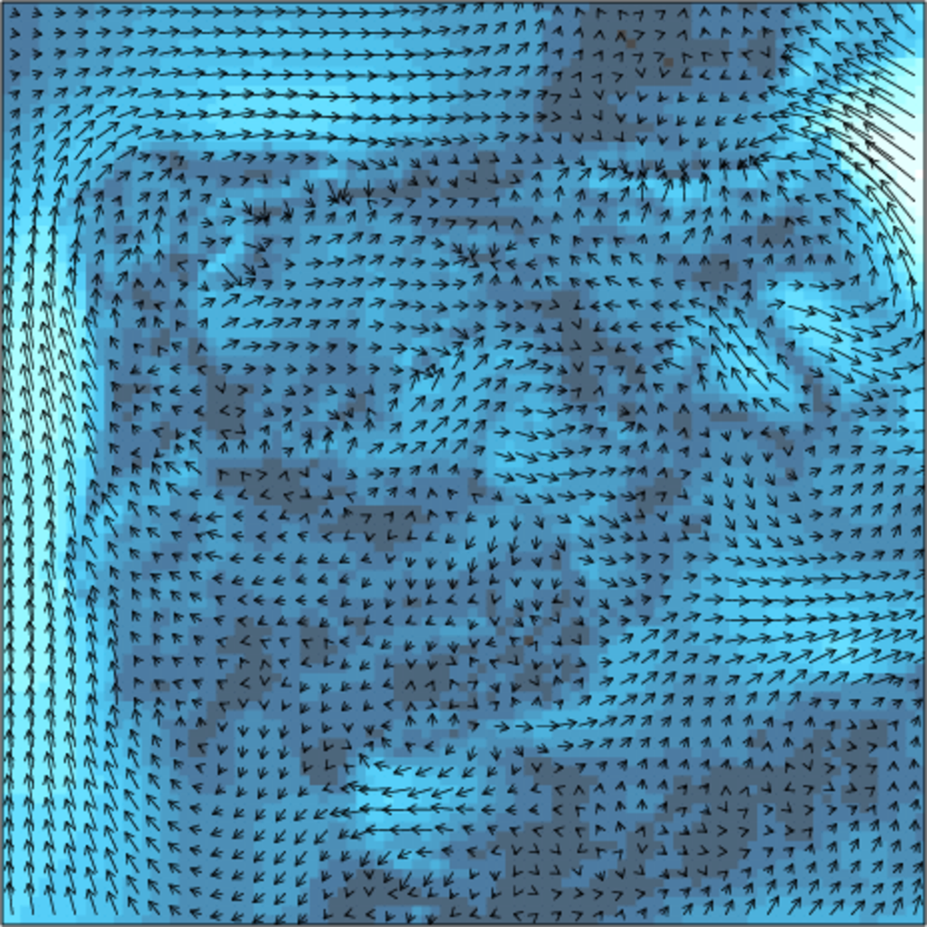
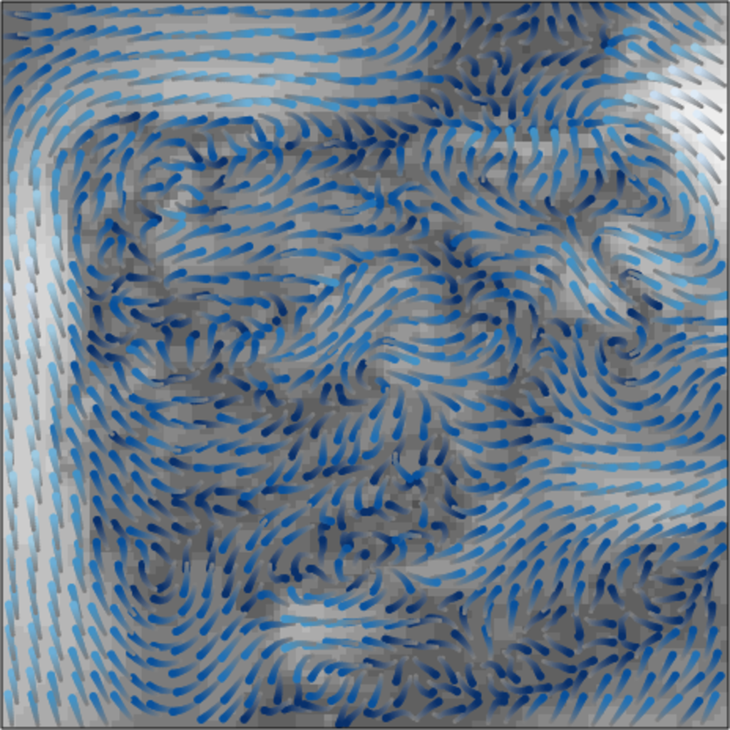
##################################################################
## Initial configuration
##################################################################
## Clone or download the repository and set the working directory
## with setwd to the folder where the repository is located.

library("raster")
library("rasterVis")
library("RColorBrewer")

## Local vector direction
wDir <- raster('data/Spatial/wDir')/180*pi
## Local vector magnitude
wSpeed <- raster('data/Spatial/wSpeed')
## Vector field encoded in a RasterStack with two layers, magnitude
## and direction
windField <- stack(wSpeed, wDir)
names(windField) <- c('magnitude', 'direction')

##################################################################
## Arrow plot
##################################################################

vectorTheme <- BTCTheme(regions = list(alpha = 0.7))

vectorplot(windField,
           isField = TRUE, ##RasterStack is a vector field
           aspX = 5, aspY = 5, ##Multipliers to adjust the relation
                               ##between slope/aspect and
                               ##horizontal/vertical displacements in
                               ##the figure.
           scaleSlope = FALSE, ## Slope values are *not* scaled
           par.settings = vectorTheme,
           colorkey = FALSE,
           scales = list(draw = FALSE))

##################################################################
## Streamlines
##################################################################

myTheme <- streamTheme(
    region = rev(brewer.pal(n = 4, "Greys")),
    symbol = rev(brewer.pal(n = 9, "Blues")))

streamplot(windField, isField = TRUE,
           par.settings = myTheme,
           droplet = list(pc = 12), ## Amount of droplets, percentage of cells
           streamlet = list(L = 5, ## Length of the streamlet
                            h = 5), ## Calculation step
           scales = list(draw = FALSE),
           panel = panel.levelplot.raster)
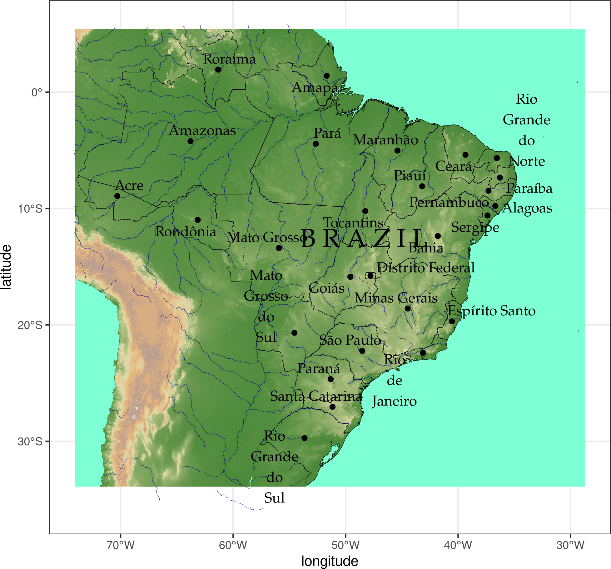
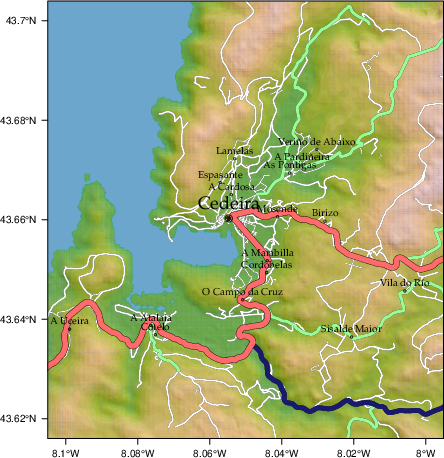
8.6. Physical maps
##################################################################
## Initial configuration
##################################################################
## Clone or download the repository and set the working directory
## with setwd to the folder where the repository is located.
library("lattice")
library("ggplot2")
## latticeExtra must be loaded after ggplot2 to prevent masking of its
## `layer` function.
library("latticeExtra")

library("RColorBrewer")

source("configLattice.R")

##################################################################
## Physical maps
##################################################################

library("terra")

library("sf")
library("sp")

library("rasterVis")
library("tidyterra")

library("colorspace")

library("ggrepel")

library("rnaturalearth")
library("rnaturalearthhires")
library("geodata")

##################################################################
## Retrieving data from DIVA-GIS, GADM and Natural Earth Data
##################################################################

     brazilAdm <- ne_states(country = "brazil")

     brazilDEM <- elevation_30s("BRA", mask = FALSE,
                                path = tempdir())

     worldRiv <- ne_download(type = "rivers_lake_centerlines",
                             category = "physical",
                             scale = 10)

     ## only those features labeled as "River" are needed
     worldRiv <- worldRiv[worldRiv$featurecla == "River",]

     ## Ensure the CRS of brazilDEM matches the CRS of worldRiv
     crs(brazilDEM) <- crs(worldRiv)

     ## and intersect it with worldRiv to extract brazilian rivers
     ## from the world database
     brazilRiv <- st_crop(worldRiv, brazilDEM)

##################################################################
## Labels
##################################################################

## Locations of labels of each polygon
centroids <- brazilAdm[ , c("longitude", "latitude")]
## Extract the data
centroids <- st_drop_geometry(centroids)
## Location of the "Brazil" label (average of the centroids)
xyBrazil <- apply(centroids, 2, mean)

admNames <- strsplit(as.character(brazilAdm$name), ' ')

admNames <- sapply(admNames,
                   FUN = function(s){
                       sep = if (length(s)>2) '\n' else  ' '
                       paste(s, collapse = sep)
                   })

##################################################################
## Overlaying layers of information
##################################################################

terrainTheme <- rasterTheme(region = terrain_hcl(15),
                            panel.background = list(col = "lightskyblue1"))

altPlot <- levelplot(brazilDEM, par.settings = terrainTheme,
                     maxpixels = 1e6, panel = panel.levelplot.raster,
                     margin = FALSE, colorkey = FALSE)

print(altPlot)

ggplot() +
  geom_spatraster(data = brazilDEM,
                  show.legend = FALSE) +
  scale_fill_whitebox_c("high_relief",
                        na.value = "aquamarine") +
  theme_bw()

brazilRivsp <- as_Spatial(brazilRiv)

brazilAdmsp <- as_Spatial(brazilAdm)

## lattice version
altPlot + layer({
  ## Rivers
  sp.lines(brazilRivsp, col = 'darkblue', lwd = 0.2)
  ## Administrative boundaries
  sp.polygons(brazilAdmsp, col = 'black', lwd = 0.2)
  ## Centroids of administrative boundaries ...
  panel.points(centroids, col = 'black')
  ## ... with their labels
  panel.text(centroids, labels = admNames, pos = 3,
             cex = 0.7, fontfamily = 'Palatino', lineheight=.8)
  ## Country name
  panel.text(xyBrazil[1], xyBrazil[2], label = 'B R A Z I L',
             cex = 1.5, fontfamily = 'Palatino', fontface = 2)
  })

## ggplot2 version
ggplot() +
  geom_spatraster(data = brazilDEM,
                  show.legend = FALSE) +
  scale_fill_whitebox_c("high_relief",
                        na.value = "aquamarine") +
  geom_sf(data = brazilAdm,
          col = "black",
          linewidth = 0.15,
          fill = "transparent") +
  geom_sf(data = brazilRiv,
          col = "darkblue",
          linewidth = 0.1) +
  geom_point(data = centroids,
                     aes(x = longitude,
                         y = latitude)) +
  geom_text_repel(data = centroids,
                          aes(x = longitude,
                              y = latitude,
                              label = admNames),
                  family = "Palatino") +
  geom_text(aes(xyBrazil[1], xyBrazil[2],
                label = 'B R A Z I L'),
            size = 7,
            family = 'Palatino') +
  theme_bw()
8.7. Data
##################################################################
## Initial configuration
##################################################################
## Clone or download the repository and set the working directory
## with setwd to the folder where the repository is located.

  ##################################################################
  ## Air Quality in Madrid
  ##################################################################

##################################################################
## Retrieve data
##################################################################

airStations <- read.csv2("data/Spatial/airStations.csv")
head(airStations)

airQuality <- read.csv2("data/Spatial/airQuality.csv")
head(airQuality)

##################################################################
## Combine data and spatial locations
##################################################################

library("sf")

## Spatial location of stations
airStations <- st_as_sf(airStations,
                        coords = c("long", "lat"),
                        crs = 4326)

NO2 <- subset(airQuality, codParam == 8)

NO2agg <- aggregate(dat ~ codEst, data = NO2,
                    FUN = function(x) {
                      c(mean = signif(mean(x), 3),
                        median = median(x),
                        sd = signif(sd(x), 3))
                    })
NO2agg <- do.call(cbind, NO2agg)
NO2agg <- as.data.frame(NO2agg)

## Link aggregated data with stations to obtain a sf object
## Code and codEst are the stations codes
idxNO2 <- match(airStations$Code, NO2agg$codEst)
NO2sf <- cbind(airStations[, c("Name", "alt")],
               NO2agg[idxNO2, ])

## Save the result
st_write(NO2sf, dsn = "data/Spatial/", layer = "NO2sf",
         driver = "ESRI Shapefile")

##################################################################
## Spanish General Elections
##################################################################

dat2016 <- read.csv("data/Spatial/GeneralSpanishElections2016.csv")

population <- dat2016$Población
census <- dat2016$Total.censo.electoral
validVotes <- dat2016$Votos.válidos
## Election results per political party and municipality
votesData <- dat2016[, -(1:13)]
## Abstention as an additional party
votesData$ABS <- census - validVotes
## UP is a coalition of several parties
UPcols <- grep("PODEMOS|ECP", names(votesData))
votesData$UP <- rowSums(votesData[, UPcols])
votesData[, UPcols] <- NULL
## Winner party at each municipality
whichMax <- apply(votesData,  1, function(x)names(votesData)[which.max(x)])
## Results of the winner party at each municipality
Max <- apply(votesData, 1, max)
## OTH for everything but PP, PSOE, UP, Cs, and ABS
whichMax[!(whichMax %in% c("PP", "PSOE", "UP", "C.s", "ABS"))] <- "OTH"
## Percentage of votes with the electoral census
pcMax <- Max/census * 100

## Province-Municipality code. sprintf formats a number with leading zeros.
PROV <- sprintf("%02d", dat2016$Código.de.Provincia)
MUN <- sprintf("%03d", dat2016$Código.de.Municipio)
PROVMUN <- paste0(PROV, MUN)

votes2016 <- data.frame(PROV, MUN, PROVMUN,
                        population, census, validVotes,
                        whichMax, Max, pcMax)

write.csv(votes2016, "data/Spatial/votes2016.csv", row.names = FALSE)

##################################################################
## Administrative boundaries
##################################################################

library("sf")

old <- setwd(tempdir())

download.file("https://www.ine.es/pcaxis/mapas_completo_municipal.zip",
              "mapas_completo_municipal.zip")
unzip("mapas_completo_municipal.zip")

sfMun <- st_read("esp_muni_0109.shp", crs = 25830,
                 stringsAsFactors = TRUE)
sfMun <- subset(sfMun, !is.na(sfMun$PROVMUN))

setwd(old)

votes2016 <- read.csv("data/Spatial/votes2016.csv",
                      colClasses = c("factor", "factor", "factor",
                                     "numeric", "numeric", "numeric",
                                     "factor", "numeric", "numeric"))
## Match polygons and data with the PROVMUN column
idx <- match(sfMun$PROVMUN, votes2016$PROVMUN)

##Places without information
idxNA <- which(is.na(idx))

##Information to be added to the sf object
dat2add <- votes2016[idx, c("PROV", "population", "census", "validVotes",
                            "whichMax", "Max", "pcMax")]

## Spatial object with votes data
sfMapVotes <- cbind(sfMun, dat2add)

## Drop those places without information
sfMapVotes0 <- sfMapVotes[-idxNA, ]

## Save the result
st_write(sfMapVotes0, "data/Spatial/sfMapVotes0.shp")

## Extract Canarias islands from the sf object
canarias <-  substr(sfMapVotes0$PROVMUN, 1, 2) %in% c("35",  "38")
peninsula <- sfMapVotes0[!canarias,]
island <- sfMapVotes0[canarias,]

## Shift the island extent box to position them at the bottom right corner
dbbox <- st_bbox(peninsula) - st_bbox(island)
dxy <- dbbox[c("xmax", "ymin")]
island$geometry <- island$geometry + dxy

## Bind Peninsula (without islands) with shifted islands
st_crs(island) <- st_crs(peninsula)
sfMapVotes <- rbind(peninsula, island)

## Save the result
st_write(sfMapVotes, "data/Spatial/sfMapVotes.shp", append = FALSE)

##################################################################
##   GDP and Population
##################################################################

## Population of each province
popSpain <- read.csv("data/SpatioTime/PopSpain.csv")
popSpain2020 <- subset(popSpain, Year == 2020)
popSpain2020$PROV <- substring(popSpain2020$Province, 1, 2)

## GDP of each province
GDPSpain2020 <- read.csv("data/Spatial/GDPSpain2020.csv")
GDPSpain2020$PROV <- substring(GDPSpain2020$Province, 1, 2)

popGDPSpain2020 <- merge(popSpain2020, GDPSpain2020[, c("PROV", "GDP")])

library("sf")

sfProv <- st_read("data/Spatial/spain_provinces_2.shp", crs = 25830,
                 stringsAsFactors = TRUE)

## Merge data with the polygons
sfPopGDPSpain <- merge(sfProv, popGDPSpain2020,
                      by = "PROV")

st_write(sfPopGDPSpain, "data/Spatial/sfPopGDPSpain.shp")

  ##################################################################
  ## CM SAF
  ##################################################################

library("raster")

tmp <- tempdir()
unzip("data/Spatial/SISmm2008_CMSAF.zip", exdir = tmp)
filesCMSAF <- dir(tmp, pattern = "SISmm")
SISmm <- stack(paste(tmp, filesCMSAF, sep = "/"))
## CM-SAF data is average daily irradiance (W/m2). Multiply by 24
## hours to obtain daily irradiation (Wh/m2)
SISmm <- SISmm * 24

## Monthly irradiation: each month by the corresponding number of days
daysMonth <- c(31, 29, 31, 30, 31, 30, 31, 31, 30, 31, 30, 31)
SISm <- SISmm * daysMonth / 1000 ## kWh/m2
## Annual average
SISav <- sum(SISm)/sum(daysMonth)
writeRaster(SISav, file = "data/Spatial/SISav.nc")

library("raster")
## https://neo.gsfc.nasa.gov/view.php?datasetId=SEDAC_POP
pop <- raster("data/Spatial/875430rgb-167772161.0.FLOAT.TIFF")
## https://neo.gsfc.nasa.gov/view.php?datasetId=MCD12C1_T1
landClass <- raster("data/Spatial/241243rgb-167772161.0.TIFF")