Spatio-temporal data - Displaying time series, spatial and space-time data with R
Table of Contents
1. Spatial point data
1.1. Graphics with spacetime

1.2. Animation


2. Spatiotemporal Areal data
3. Spatiotemporal Raster data
3.1. Level plots
3.2. Graphical Exploratory Data Analysis

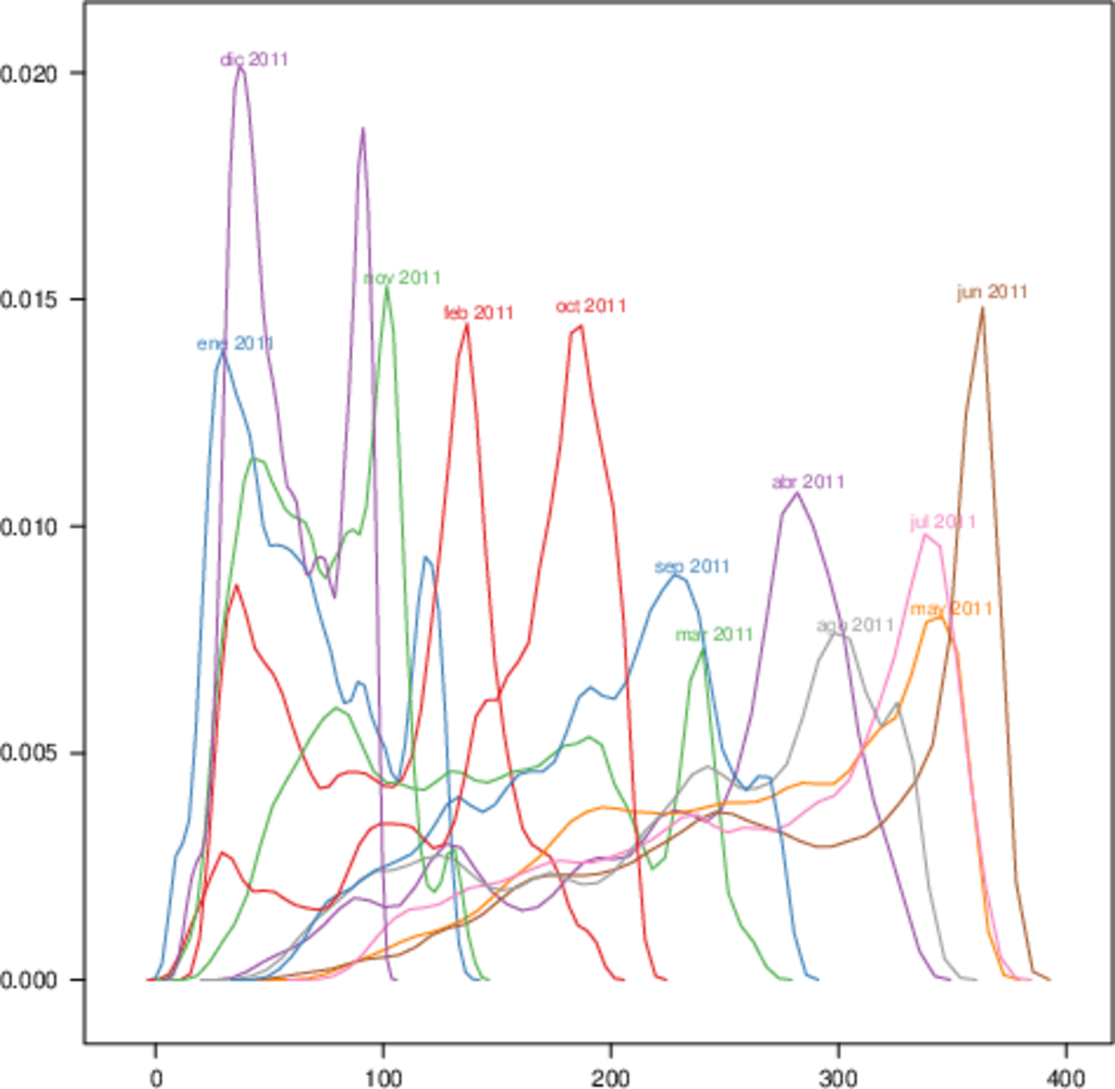

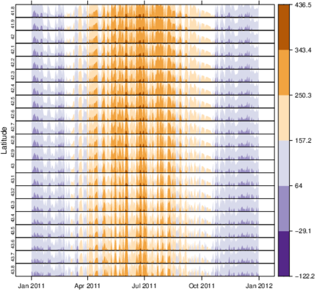
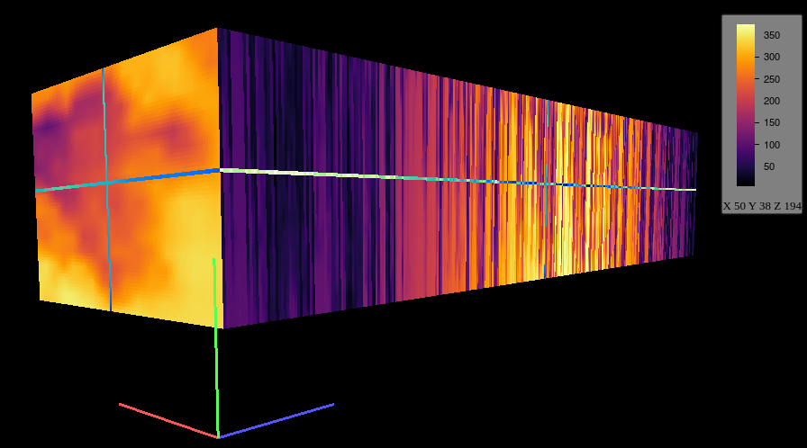
3.3. Space-Time and Time Series Plots

3.4. Animation
4. Animation
5. Code
5.1. Spatiotemporal point data
##################################################################
## Initial configuration
##################################################################
## Clone or download the repository and set the working directory
## with setwd to the folder where the repository is located.
library("lattice")
library("ggplot2")
## latticeExtra must be loaded after ggplot2 to prevent masking of its
## `layer` function.
library("latticeExtra")

library("RColorBrewer")

source('configLattice.R')

Sys.setlocale("LC_TIME", "C")

##################################################################
## Data and spatial information
##################################################################

## Spatial location of stations
airStations <- read.csv2("data/Spatial/airStations.csv")
## Measurements data
airQuality <- read.csv2("data/Spatial/airQuality.csv")
## Only interested in NO2
NO2 <- airQuality[airQuality$codParam == 8, ]

library("zoo")
library("reshape2")

library("sp")
library("spacetime")

library("sf")
library("sftime")

##################################################################
## sp and spacetime
##################################################################

airStationsSP <- airStations
## rownames are used as the ID of the Spatial object
rownames(airStationsSP) <- substring(airStationsSP$Code, 7)
coordinates(airStationsSP) <- ~ long + lat
proj4string(airStationsSP) <- CRS("+proj=longlat +ellps=WGS84")

NO2$time <- as.Date(with(NO2,
                         ISOdate(year, month, day)))

NO2wide <- dcast(NO2[, c('codEst', 'dat', 'time')],
                 time ~ codEst,
                 value.var = "dat")

NO2zoo <- zoo(NO2wide[,-1], NO2wide$time)

dats <- data.frame(vals = as.vector(t(NO2zoo)))

NO2st <- STFDF(sp = airStationsSP,
               time = index(NO2zoo),
               data = dats)

##################################################################
## sf and sftime
##################################################################

airStationsSF <- st_as_sf(airStations,
                          coords = c("long", "lat"),
                          crs = 4326)

NO2$time <- as.Date(with(NO2,
                         ISOdate(year, month, day)))

idx <- match(NO2$codEst, airStationsSF$Code)

NO2sft <- st_sftime(dat = NO2$dat, code = NO2$codEst,
                    geometry = airStationsSF$geometry[idx],
                    time = NO2$time)

##################################################################
## Graphics with spacetime and sftime
##################################################################

airPal <- colorRampPalette(c("springgreen1", "sienna3", "gray5"))(5)

stplot(NO2st[, 1:12],
       cuts = 5,
       col.regions = airPal,
       main = "",
       edge.col = "black")

airPal <- colorRampPalette(c("springgreen1", "sienna3", "gray5"))(5)

ggplot(NO2sft) +
  geom_sf(aes(color = dat)) +
  facet_wrap(~ cut(time, 12)) +
  scale_colour_stepsn(n.breaks = 6, colours = airPal)

stplot(NO2st, mode = "xt",
       col.regions = colorRampPalette(airPal)(15),
       scales = list(x = list(rot = 45)),
       ylab = "", xlab = "", main = "")

ggplot(NO2sft) +
  geom_tile(aes(x = as.factor(code),
                y = time,
                fill = dat)) +
  scale_fill_stepsn(colours = airPal,
                    n.breaks = 6) +
  xlab("Station Code") + ylab("") +
  guides(x = guide_axis(angle = 45))

stplot(NO2st, mode = "ts",
       xlab = "",
       lwd = 0.1, col = "black", alpha = 0.6,
       auto.key = FALSE)

ggplot(NO2sft) +
  geom_line(aes(x=time, y = dat),
            colour = "black",
            linewidth = 0.25,
            alpha = 0.6) +
  theme_bw() + xlab("")

##################################################################
## Point space-time data
##################################################################

##################################################################
## Initial snapshot
##################################################################

library("sp")
library("zoo")
library("reshape2")
library("spacetime")

airStationsSP <- read.csv2("data/Spatial/airStations.csv")
rownames(airStationsSP) <- substring(airStationsSP$Code, 7)
coordinates(airStationsSP) <- ~ long + lat
proj4string(airStationsSP) <- CRS("+proj=longlat +ellps=WGS84")
airQuality <- read.csv2("data/Spatial/airQuality.csv")
NO2 <- airQuality[airQuality$codParam == 8, ]

NO2$time <- as.Date(with(NO2,
                         ISOdate(year, month, day)))

NO2wide <- dcast(NO2[, c("codEst", "dat", "time")],
                 time ~ codEst,
                 value.var = "dat")

NO2zoo <- zoo(NO2wide[,-1], NO2wide$time)

dats <- data.frame(vals = as.vector(t(NO2zoo)))

NO2st <- STFDF(sp = airStationsSP,
               time = index(NO2zoo),
               data = dats)

library("grid")
library("gridSVG")

## Initial parameters
start <- NO2st[,1]
## values will be encoded as size of circles,
## so we need to scale them
startVals <- start$vals/5000

nStations <- nrow(airStationsSP)
days <- index(NO2zoo)
nDays <- length(days)
## Duration in seconds of the animation
duration <- nDays*.3

## Auxiliary panel function to display circles
panel.circlesplot <- function(x, y, cex, col = "gray",
                              name = "stationsCircles", ...) {
  grid.circle(x, y, r = cex,
              gp = gpar(fill = col, alpha = 0.5),
              default.units = "native", name = name)
}

pStart <- spplot(start, panel = panel.circlesplot,
                 cex = startVals,
                 scales = list(draw = TRUE), auto.key = FALSE)
pStart

##################################################################
## Intermediate states to create the animation
##################################################################

## Color to distinguish between weekdays ('green') and weekend
## ('blue')
isWeekend <- function(x) {format(x, "%w") %in% c(0, 6)}
color <- ifelse(isWeekend(days), "blue", "green")
colorAnim <- animValue(rep(color, each = nStations),
                       id = rep(seq_len(nStations), nDays))

## Intermediate sizes of the circles
vals <- NO2st$vals/5000
vals[is.na(vals)] <- 0
radius <- animUnit(unit(vals, "native"),
                   id = rep(seq_len(nStations), nDays))

## Animation of circles including sizes and colors
grid.animate("stationsCircles",
             duration = duration,
             r = radius,
             fill = colorAnim,
             rep = TRUE)

##################################################################
## Time reference: progress bar
##################################################################

## Progress bar
prettyDays <- pretty(days, 12)
## Width of the progress bar
pbWidth <- .95
## Background
grid.rect(.5, 0.01, width = pbWidth, height = .01,
          just = c("center", "bottom"),
          name = "bgbar", gp = gpar(fill = "gray"))

## Width of the progress bar for each day
dayWidth <- pbWidth/nDays
ticks <- c(0, cumsum(as.numeric(diff(prettyDays)))*dayWidth) + .025
grid.segments(ticks, .01, ticks, .02)
grid.text(format(prettyDays, "%d-%b"),
          ticks, .03, gp = gpar(cex = .5))
## Initial display of the progress bar
grid.rect(.025, .01, width = 0,
          height = .01, just = c("left", "bottom"),
          name = "pbar", gp = gpar(fill = "blue", alpha = ".3"))
## ...and its animation
grid.animate("pbar", duration = duration,
             width = seq(0, pbWidth, length = duration),
             rep = TRUE)
## Pause animations when mouse is over the progress bar
grid.garnish("bgbar",
             onmouseover = "document.documentElement.pauseAnimations()",
             onmouseout = "document.documentElement.unpauseAnimations()")

grid.export("figs/SpatioTime/NO2pb.svg")

##################################################################
## Time reference: a time series plot
##################################################################

library("lattice")
library("latticeExtra")

## Time series with average value of the set of stations
NO2mean <- zoo(rowMeans(NO2zoo, na.rm = TRUE), index(NO2zoo))
## Time series plot with position highlighted
pTimeSeries <- xyplot(NO2mean, xlab = "", identifier = "timePlot") +
  layer({
    grid.points(0, .5, size = unit(.5, "char"),
                default.units = "npc",
                gp = gpar(fill = "gray"),
                name = "locator")
    grid.segments(0, 0, 0, 1, name = "vLine")
  })

print(pStart, position = c(0, .2, 1, 1), more = TRUE)
print(pTimeSeries, position = c(.1, 0, .9, .25))

grid.animate("locator",
             x = unit(as.numeric(index(NO2zoo)), "native"),
             y = unit(as.numeric(NO2mean), "native"),
             duration = duration, rep = TRUE)

xLine <- unit(index(NO2zoo), "native")

grid.animate("vLine",
             x0 = xLine, x1 = xLine,
             duration = duration, rep = TRUE)

grid.animate("stationsCircles",
             duration = duration,
             r = radius,
             fill = colorAnim,
             rep = TRUE)

## Pause animations when mouse is over the time series plot
grid.garnish("timePlot", grep = TRUE,
             onmouseover = "document.documentElement.pauseAnimations()",
             onmouseout = "document.documentElement.unpauseAnimations()")

grid.export("figs/SpatioTime/vLine.svg")
5.2. Spatiotemporal areal data
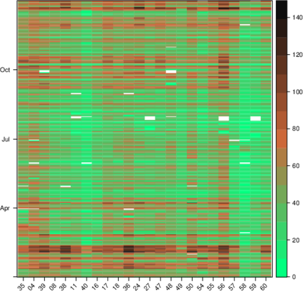
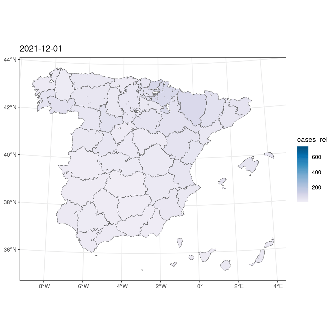
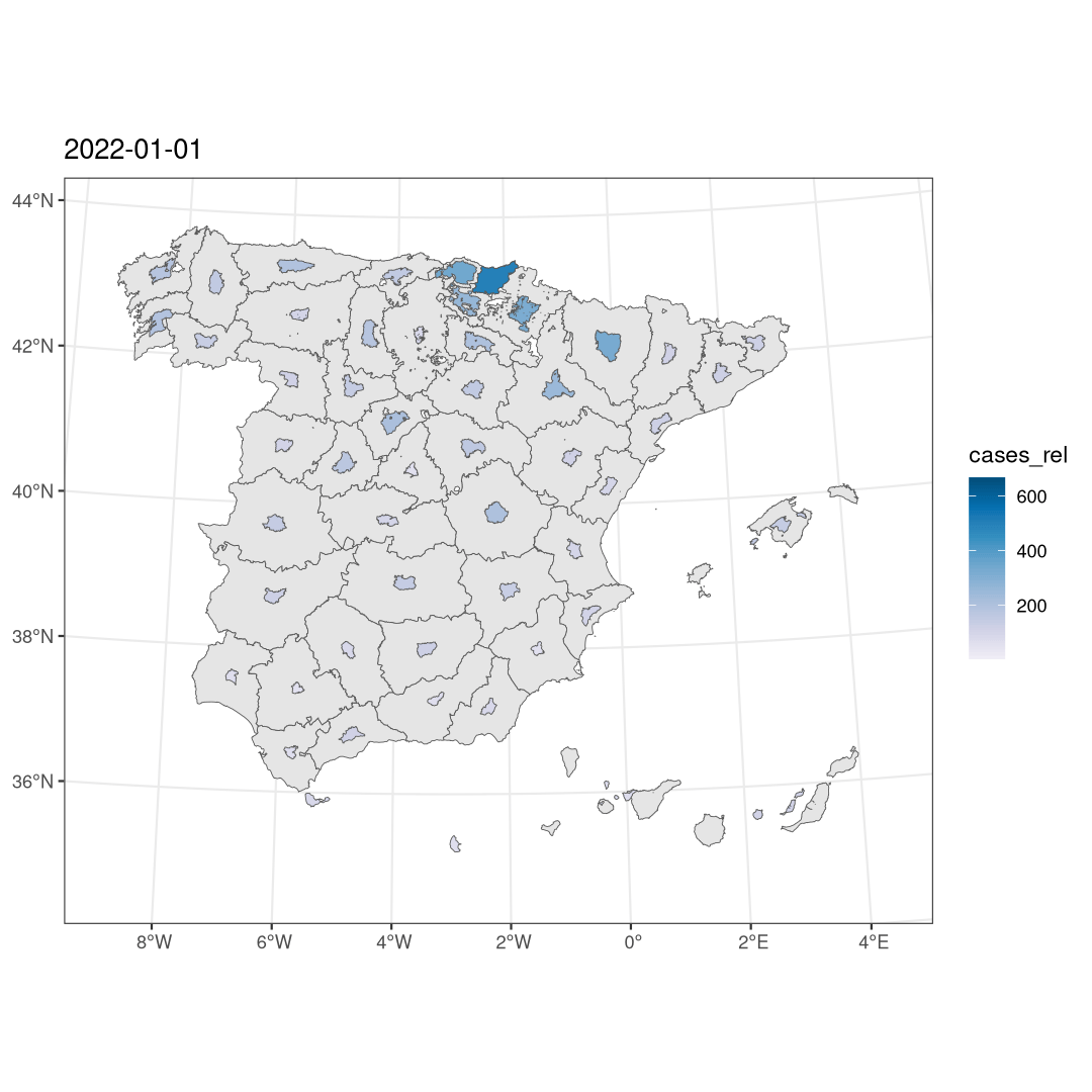
##################################################################
## Initial configuration
##################################################################
## Clone or download the repository and set the working directory
## with setwd to the folder where the repository is located.
Sys.setlocale("LC_TIME", "C")

##################################################################
## Data and spatial information
##################################################################

library("sf")

library("cartogram")

library("gganimate")

covidSpain <- read.csv("data/SpatioTime/covid.csv",
                       na.strings = NULL)
covidSpain$PROV <- sprintf("%02d", covidSpain$PROV)
covidSpain$day <- as.Date(covidSpain$day)

covidSpain <- subset(covidSpain,
                     day < as.Date("2022-03-01") &
                     day >= as.Date("2021-12-01"))

## Population of each province
popSpain <- read.csv("data/SpatioTime/PopSpain.csv")
popSpain$PROV <- substring(popSpain$Province, 1, 2)

popSpain2021 <- subset(popSpain,
                       Year == 2021,
                       select = c(PROV, Population))

covidSpain <- merge(covidSpain, popSpain2021, by = "PROV")

## Number of cases per 100.000 population
covidSpain$cases_rel <- with(covidSpain,
                             num_cases/Population * 1e5)

ggplot(covidSpain) +
  geom_raster(aes(x = day,
                  y = PROV,
                  fill = cases_rel)) +
  scale_fill_distiller(palette = "PuBu", direction = 1) +
  theme_bw()

sfProv <- st_read("data/Spatial/spain_provinces_2.shp",
                  crs = 25830,
                  stringsAsFactors = TRUE)

## Merge data with the polygons
sfCovid <- merge(sfProv, covidSpain,
                      by = "PROV")

ggplot(subset(sfCovid,
              day >= as.Date("2022-01-01") &
              day <= as.Date("2022-01-09"))) +
  geom_sf(aes(fill = cases_rel)) +
  scale_fill_distiller(palette = "PuBu", direction = 1) +
  theme_bw() +
  facet_wrap(~ day, nrow = 3)

ggCovid <- ggplot(sfCovid) +
  geom_sf(aes(fill = cases_rel)) +
  scale_fill_distiller(palette = "PuBu", direction = 1) +
  theme_bw() +
  ggtitle("{format(frame_time, format = '%Y-%m-%d')}") +
  transition_time(time = day)


animate(ggCovid,
        height = 1080, width = 1080,
        res = 150,
        units = "px")

fday <- as.Date("2022-01-01")
lday <- as.Date("2022-02-28")

days <- seq(fday, lday, by = "day")

cartCOVIDList <- lapply(days, function(d)
{
  x <- subset(sfCovid, day == d)
  cartogram_ncont(x,
                  weight = "cases_rel")
})
cartCOVID <- do.call(rbind, cartCOVIDList)

ggplot(subset(cartCOVID,
              day >= as.Date("2022-01-01") &
              day <= as.Date("2022-01-09"))) +
  geom_sf(data = sfProv) +
  geom_sf(aes(fill = cases_rel)) +
  scale_fill_distiller(palette = "PuBu", direction = 1) +
  theme_bw() +
  facet_wrap(~ day, nrow = 3)

ggCartCOVID <- ggplot(cartCOVID) +
  geom_sf(data = sfProv) +
  geom_sf(aes(fill = cases_rel, group = day)) +
  scale_fill_distiller(palette = "PuBu", direction = 1) +
  ggtitle("{format(frame_time)}") +
  transition_time(day) +
  theme_bw()


animate(ggCartCOVID,
        height = 1080, width = 1080,
        res = 150,
        units = "px")
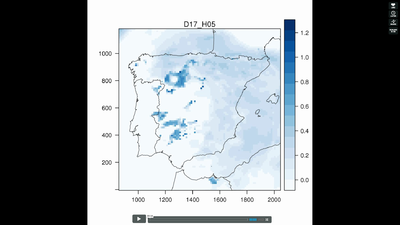
5.3. Spatiotemporal raster data
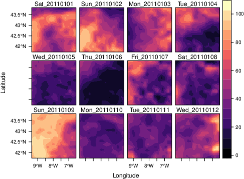
##################################################################
## Initial configuration
##################################################################
## Clone or download the repository and set the working directory
## with setwd to the folder where the repository is located.

Sys.setlocale("LC_TIME", "C")

library("raster")
library("terra")

library("zoo")

library("RColorBrewer")
library("rasterVis")

SISdm <- brick("data/SpatioTime/SISgal")

timeIndex <- seq(as.Date("2011-01-01"), by = "day", length = 365)
SISdm <- setZ(SISdm, timeIndex)
names(SISdm) <- format(timeIndex, "%a_%Y%m%d")

SISdmt <- rast(SISdm)
time(SISdmt) <- timeIndex

##################################################################
## Levelplot
##################################################################

levelplot(SISdm, layers = 1:12, panel = panel.levelplot.raster)

SISmm <- zApply(SISdm, by = as.yearmon, fun = 'mean')

levelplot(SISmm, panel = panel.levelplot.raster)

##################################################################
## Exploratory graphics
##################################################################

histogram(SISdm, FUN = as.yearmon)

bwplot(SISdm, FUN = as.yearmon)

splom(SISmm, xlab = '', plot.loess = TRUE)

##################################################################
## Space-time and time series plots
##################################################################

hovmoller(SISdm)

xyplot(SISdm, auto.key = list(space = 'right'))

horizonplot(SISdm, digits = 1,
            col.regions = rev(brewer.pal(n = 6, 'PuOr')),
            xlab = '', ylab = 'Latitude')

library("cubeview")

## cubeview has problems if the Raster*
## is not stored in memory
SISdm <- readAll(SISdm)

cubeview(SISdm)

##################################################################
## Data
##################################################################

library("raster")
library("rasterVis")

cft <- brick("data/SpatioTime/cft_20130417_0000.nc")
## set projection
projLCC2d <- "+proj=lcc +lon_0=-14.1 +lat_0=34.823 +lat_1=43 +lat_2=43 +x_0=536402.3 +y_0=-18558.61 +units=km +ellps=WGS84"
projection(cft) <- projLCC2d
##set time index
timeIndex <- seq(as.POSIXct("2013-04-17 01:00:00", tz = "UTC"), length = 96, by = "hour")
cft <- setZ(cft, timeIndex)
names(cft) <- format(timeIndex, "D%d_H%H")

##################################################################
## Spatial context: administrative boundaries
##################################################################

library("rnaturalearth")
library("sf")
library("sp")

world <- ne_countries(scale = "medium")
## Project the extent of the cft raster to longitude-latitude, because
## rnaturalearth works with it.
cftLL <- projectExtent(cft, crs(world))
## Crop...
boundaries <- st_crop(world, cftLL)
## ... and project to the projection of the cft object
boundaries <- st_transform(boundaries, crs(cft))
## Finally, convert to a Spatial* object
boundaries <- as(boundaries, "Spatial")

##################################################################
## Producing frames and movie
##################################################################

library("RColorBrewer")
library("latticeExtra")

cloudTheme <- rasterTheme(region = brewer.pal(n = 9, 'Blues'))

tmp <- tempdir()
trellis.device(png, file = paste0(tmp, "/Rplot%02d.png"),
               res = 300, width = 1500, height = 1500)
levelplot(cft, layout = c(1, 1),
          par.settings = cloudTheme,
          scales=list(draw=FALSE)) +
  layer(sp.lines(boundaries, lwd = 0.6))
dev.off()

old <- setwd(tmp)
## Create a movie with ffmpeg ...
system2("ffmpeg",
        c("-r 6", ## with 6 frames per second
          "-i Rplot%02d.png", ## using the previous files
          "-b:v 300k", ## with a bitrate of 300kbs
          "output.mp4")
        )
file.remove(dir(pattern = "Rplot"))
file.copy("output.mp4", paste0(old, "/figs/SpatioTime/cft.mp4"), overwrite = TRUE)
setwd(old)

##################################################################
## Static image
##################################################################

levelplot(cft,
          layers = 25:48, ## Layers to display (second day)
          layout = c(6, 4), ## Layout of 6 columns and 4 rows
          par.settings = cloudTheme,
          scales=list(draw=FALSE),
          names.attr = paste0(sprintf("%02d", 1:24), "h"),
          panel = panel.levelplot.raster) +
  layer(sp.lines(boundaries, lwd = 0.6))

library("rgl")

clear3d()

pal <- colorRampPalette(brewer.pal(n = 9, "Blues"))

N <- nlayers(cft)

ids <- lapply(seq_len(N),
              FUN = function(i)
                  plot3D(cft[[i]],
                         maxpixels = 1e3,
                         col = pal,
                         adjust = FALSE, ## Disable automatic scaling of xy axes.
                         zfac = 200)) ## Common z scale for all graphics

library("manipulateWidget")

rglwidget() %>%
  playwidget(start = 0, stop = N,
             subsetControl(1, subsets = ids))
5.4. Animation
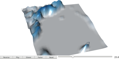
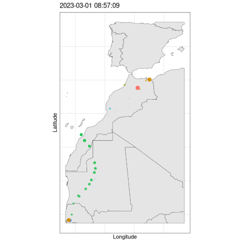
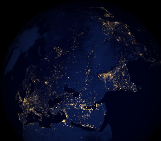
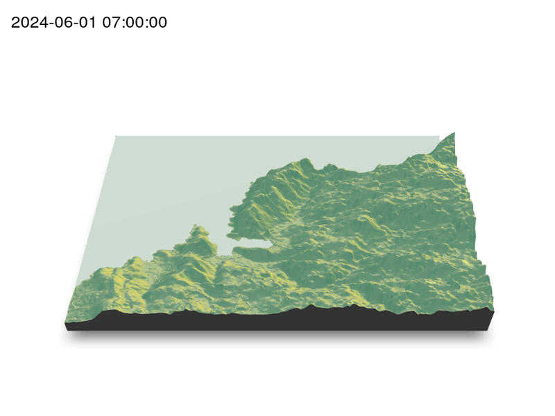
##################################################################
## Initial configuration
##################################################################
## Clone or download the repository and set the working directory
## with setwd to the folder where the repository is located.

Sys.setlocale("LC_TIME", 'C')

##################################################################
## Time trajectory
##################################################################

library("sf")
library("move2")
library("units")

library("rnaturalearth")

library("ggplot2")
library("gganimate")

## Movebank data
birds0 <- movebank_download_study(2398637362,
                                 "license-md5"="74263192947ce529c335a0ae72d7ead7")

sf_use_s2(FALSE) ## Needed for st_crop to work
## Natural Earth boundaries
boundaries <- ne_countries(scale = "large")
boundaries <- st_crop(boundaries, birds0)

## Filter the data: speed higher than 2 m/s; remove year 2022 data.
birds <- subset(birds0,
                ground_speed > set_units(2L, "m/s") &
                timestamp >= as.POSIXct("2023-01-01"))

## Add a column with month values
birds$month <- as.numeric(format(mt_time(birds), "%m"))

ggplot() +
    geom_sf(data = boundaries) +
    geom_sf(data = birds,
            aes(color = individual_local_identifier),
            alpha = 0.1) +
    guides(colour = guide_legend(override.aes = list(alpha = 1))) +
    theme_linedraw() +
    facet_wrap(~ month, nrow = 2)

birds$speed <- cut(birds$ground_speed,
                   breaks = c(2, 5, 10, 15, 35))
ggplot() +
    coord_polar(start = 0) +
    geom_histogram(data = birds,
                   aes(x = set_units(heading, "degrees"),
                       fill = speed),
                   breaks = set_units(seq(0, 360, by = 10L), "degrees"),
                   position = position_stack(reverse = TRUE)) +
    scale_x_units(name = NULL,
                  limits = set_units(c(0L, 360), "degrees"),
                  breaks = (0:4) * 90L) +
    ylab("") +
    facet_wrap(~ month, nrow = 2) +
    scale_fill_ordinal("Speed") +
    theme_linedraw()

birdsMarch <- subset(birds,
                      month == 3)
p <- ggplot() +
    geom_sf(data = boundaries) +
    geom_sf(data = birdsMarch,
            aes(colour = individual_local_identifier),
            size = 3) +
    theme_bw() +
    xlab("Longitude") + ylab("Latitude") +
    ggtitle("{format(frame_time, format = '%Y-%m-%d %H:%M:%S')}") +
    transition_time(timestamp) +
    shadow_wake(0.8)

animate(p, nframes = 300)

##################################################################
## Fly-by animation
##################################################################

library("rgl")
library("magick") ## needed to import the texture

## Opens the OpenGL device with a black background
open3d()
bg3d("black")

## XYZ coordinates of a sphere
lat <- seq(-90, 90, len = 100) * pi/180
long <- seq(-180, 180, len = 100) * pi/180
r <- 6378.1 # radius of Earth in km
x <- outer(long, lat, FUN = function(x, y) r * cos(y) * cos(x))
y <- outer(long, lat, FUN = function(x, y) r * cos(y) * sin(x))
z <- outer(long, lat, FUN = function(x, y) r * sin(y))

## Read, scale, and convert the image
nightLightsJPG <- image_read("https://eoimages.gsfc.nasa.gov/images/imagerecords/79000/79765/dnb_land_ocean_ice.2012.13500x6750.jpg")
nightLightsJPG <- image_scale(nightLightsJPG, "8192") ## surface3d reads files up to 8192x8192
nightLights <- image_write(nightLightsJPG, tempfile(),
                           format = "png") ## Only the png format is supported
## Display the sphere with the image superimposed
surface3d(-x, -z, y,
          texture = nightLights,
          specular = "black", col = "white")

rglwidget()

cities <- rbind(c("Madrid", "Spain"),
                c("Tokyo", "Japan"),
                c("Sidney", "Australia"),
                c("Sao Paulo", "Brazil"),
                c("New York", "USA"))
cities <- as.data.frame(cities)
names(cities) <- c("city", "country")

library("osmdata")

geocode <- function(x) {
  place <- paste(x, collapse = ", ")
  bb <- getbb(place)
  center <- c(sum(bb[1, ])/2, sum(bb[2, ]/2))
  center
}

points <- apply(cities, 1, geocode)
points <- t(points)
colnames(points) <- c("lon", "lat")

cities <- cbind(cities, points)

library("geosphere")

## When arriving or departing include a progressive zoom with 100
## frames
zoomIn <- seq(.3, .1, length = 100)
zoomOut <- seq(.1, .3, length = 100)

## First point of the route
route <- data.frame(lon = cities[1, "lon"],
                    lat = points[1, "lat"],
                    zoom = zoomIn,
                    name = cities[1, "city"],
                    action = "arrive")

## This loop visits each location included in the "points" set
## generating the route.
for (i in 1:(nrow(cities) - 1)) {

  p1 <- cities[i,]
  p2 <- cities[i + 1,]
  ## Initial location
  departure <- data.frame(lon = p1$lon,
                          lat = p1$lat,
                          zoom = zoomOut,
                          name = p1$city,
                          action = "depart")

  ## Travel between two points: Compute 100 points between the
  ## initial and the final locations.
  routePart <- gcIntermediate(p1[, c("lon", "lat")],
                              p2[, c("lon", "lat")],
                              n = 100)
  routePart <- data.frame(routePart)
  routePart$zoom <- 0.3
  routePart$name <- ""
  routePart$action <- "travel"

  ## Final location
  arrival <- data.frame(lon = p2$lon,
                        lat = p2$lat,
                        zoom = zoomIn,
                        name = p2$city,
                        action = "arrive")
  ## Complete route: initial, intermediate, and final locations.
  routePart <- rbind(departure, routePart, arrival)
  route <- rbind(route, routePart)
}

## Close the travel
route <- rbind(route,
               data.frame(lon = cities[i + 1, "lon"],
                          lat = cities[i + 1, "lat"],
                          zoom = zoomOut,
                          name = cities[i+1, "city"],
                          action = "depart"))

summary(route)

## Function to move the viewpoint in the RGL scene according to the
## information included in the route (position and zoom).
travel <- function(tt) {
  point <- route[tt,]
  view3d(theta = -90 + point$lon,
         phi = point$lat,
         zoom = point$zoom)
  par3d()
}

## Example of usage of travel
## Frame no.1200
travel(1200)
rgl.snapshot("figs/SpatioTime/rgl_travel1200.png")

movie3d(travel,
        duration = nrow(route),
        startTime = 1, fps = 1,
        type = "mp4", clean = FALSE,
        webshot = FALSE)

##################################################################
## Hill shading animation
##################################################################

library("rayshader")
library("parallel")
library("suntools")
library("raster")
library("gifski")

demCedeira <- raster('data/Spatial/demCedeira')
DEM <- raster_to_matrix(demCedeira)

water <- detect_water(DEM)

lonlat <- matrix(c((xmax(demCedeira) + xmin(demCedeira))/2,
                   (ymax(demCedeira) + ymin(demCedeira))/2),
                 nrow = 1)

tt <- seq(as.POSIXct("2024-06-01 07:00:00", tz = "Europe/Madrid"),
          as.POSIXct("2024-06-01 21:00:00", tz = "Europe/Madrid"),
          by = "15 min")
sun <- lapply(tt, function(x) solarpos(lonlat, x))

ncores <- detectCores()

hillshades <- mclapply(sun, function(ang)
{
    DEM %>%
        sphere_shade(texture = "imhof1", sunangle = ang[1]) %>%
        add_water(water, color = "imhof1") %>%
        add_shadow(ray_shade(DEM,
                             sunangle = ang[1],
                             sunaltitude = ang[2]),
                   0.75)
}, mc.cores = ncores)

old <- setwd(tempdir())

idx <- seq_along(hillshades)

for(i in idx)
{
    plot_3d(heightmap = DEM,
            hillshade = hillshades[[i]],
            zscale = 5,
            fov = 45,
            theta = 0,
            zoom = 0.75,
            phi = 45,
            windowsize = c(1000, 800))
    render_snapshot(filename = paste0(i, ".png"),
                    title_text = tt[i])
}

gifski(png_files = paste0(idx, ".png"),
       gif_file = "cedeira.gif",
       delay = 1/5)

setwd(old)